
Supervised Learning EP2 - An introduction to Deep Learning
Published:
Deep learning is a subfield of machine learning that involves training artificial neural networks with multiple layers to analyze and solve complex problems. These neural networks are capable of learning hierarchical representations of data, enabling them to extract features and patterns from raw input data. Deep learning has been used in a wide range of applications such as image recognition, natural language processing, and autonomous driving. This blog covers the basics of four different types of DL models, paves the way to further in-depth study of various DNN.
Multi-layer Perceptron
CLICK ME
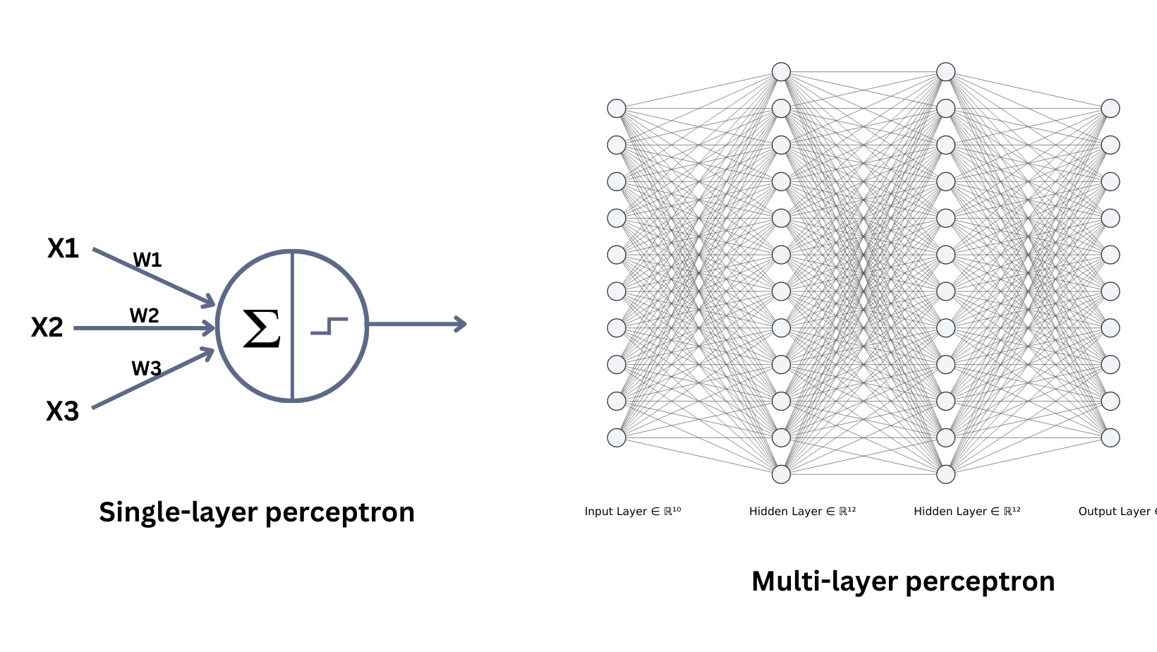
Multi-Layer Perceptron (MLP) is a type of feedforward artificial neural network (ANN) that consists of multiple layers of interconnected neurons. The output of each neuron in a layer is then passed on to the next layer, and this process continues through all the layers in the architecture. MLPs have shown great success in many artificial intelligence applications, such as image recognition, natural language processing, and speech recognition.Let's review the single layer perceptron first. The perceptron model does a weighted sum operation to an input instance $x$ and uses sign function (activation function) to generate final classification results. MLP expands perceptron by applying different activation functions and sets the output from current perceptron as the input to the next perceptron. Layers between input layer and output layer is called hidden layers, which contain non-linear activation functions.
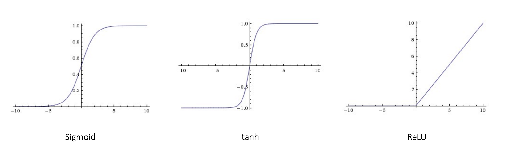
Several commonly used activation functions: 1. Sigmoid $$ f(x)=\frac{1}{1+exp(-x)}\\ f^{\prime}(x)=\frac{exp(-x)}{(1+exp(-x))^2}=f(x)(1-f(x)) $$ 2. Rectified linear unit (Relu) $$ f(x)= \begin{cases} x, x \geq 0\\[1ex] 0, x \lt 0 \end{cases}\\ f^{\prime}(x)=\begin{cases} 1, x \geq 0\\[1ex] 0, x \lt 0 \end{cases} $$ 3. Tanh $$ f(x)=\frac{2}{1+exp(-2x)}-1\\ f^{\prime}(x)=\frac{4 exp(-2x)}{(1+exp(-2x))^2}=1-f(x)^2 $$
How to set the number of layers and number of neurons per layer? So far we have not found one model structure that fits all problems, we can find a suitable architecture for a specific task using neural architecture search (NAS). Modern deep neural networks usually have tens or hundreds of layers, although we have Universality Approximation Theorem: 2-layer net with linear output with some squashing non-linearity in hidden units can approximate any continuous function over compact domain to arbitrary accuracy (given enough hidden units!)
Convolutional Neural Network
CLICK ME
Convolutional neural networks (CNN) are simply neural networks that use convolution in place of general matrix multiplication in at least one of their layers. CNNs are known for their ability to extract features from images, and they can be trained to recognize patterns within them. You may heard of convolution in signal processing. For 2-D image signal, convolution operation can be written as: $$ f(x,y)=(g*k)(x,y)=\sum_{m} \sum_{n} g(i-m,i-n) k(m,n) $$ where $*$ is convolution operation, $g$ is 2-D image data and $k$ is convolution kernel. First rotate the convolution kernel 180 degrees clockwise, and then do element-wise dot production. In fact, convolution in CNN is not the same convolution operation as mentioned above. It is actually a correlation operation, which directly perform element-wise dot production between kernel and image patches.In a CNN with multiple layers, neurons in a layer are only connected to a small region of the layer before it, which is so-called local connectivity. One kernel matrix or kernel map is shared between all the patches of an image, namely weight sharing, which allows to learn shift-invariant filter kernels (same feature would be recognized no matter it's location in an image, e.g. a cat will be detected no matter it's on the top left or in the middle of the image) and reduce the number of parameters.
Apart from convolutional layers, the design of CNNs involves operations such as pooling layers, non-linearity and fully connected layers. The convolutional layers are responsible for applying filters for feature extraction to the input image, while the pooling layers then reduce the size of the feature map produced by the convolutional layers, and expand the receptive field from local to global. Finally, the fully connected layers are used to generate prediction result based on the features extracted by the CNN. Take Vgg16 as an example.
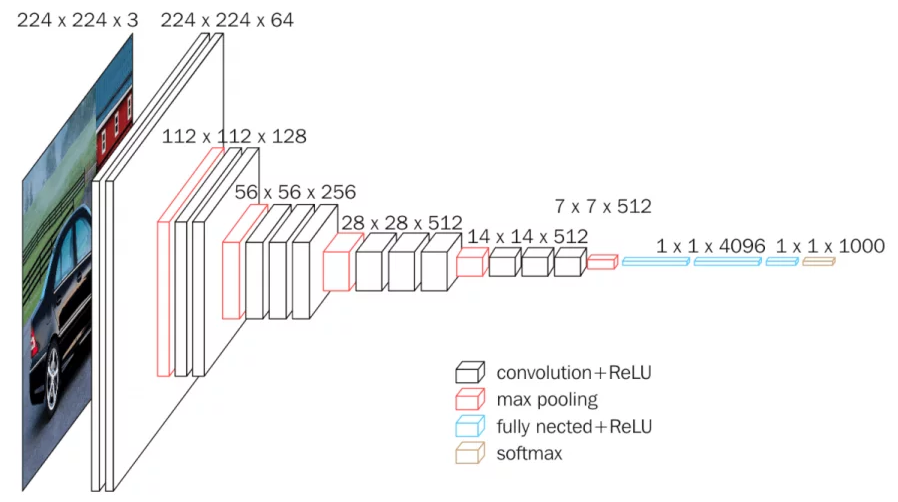
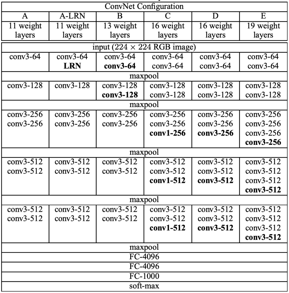
Given a three channel input image (RGB) with size 224 $\times$ 224, Vgg16 first resizes it to 225 $\times$ 225 by adding pixels to the input image (padding, usually fill in zero value pixels around the image), and perform convolution using 64 3 $\times$ 3 conv kernels or filters (obtain 64 feature maps,i.e. output 64 channels, with size 224 $\times$ 224) and Relu. Padding is to keep the size of feature map same as the input image, since the size will be smaller than 224 $\times$ 224 after convolution without padding. Perform the same convolution again, then shrink the feature map size to 112 $\times$ 112 by maxpooling, which picks the maximum of 2 $\times$ 2 square pixel patch as the output pixel value to halve the side length. Repeat conv+Relu+maxpool, followed by three fully connected layers and softmax (predict the probability of each class). Here's the configuration of vgg convnets.
Now let's calculate the number of parameters used in a convolution layer and a fully connected layer, to get a better understanding of how a CNN works. A 3 $\times$ 3 conv kernel has 9 parameters. The first convolution layer uses 64 kernels with size 3 $\times$ 3 to process a 3-channel image, which has 3 $\times$ 3 $\times$ 3 $\times$ 64 parameters. We can regard it as a cube kernel with size 3 $\times$ 3 $\times$ 3, obtained by multiplying kernel size and input channels. **Parameter amount = (conv kernel size * the number of channels of the input feature map) * the number of conv kernels**. The feature map obtained by the last convolution of VGG-16 is 7 $\times$ 7 $\times$ 512, which is expanded into a one-dimensional vector 1 $\times$ 4096 by the first fully connected layer. How to do that? We actually employ 4096 cube kernels with size 7 $\times$ 7 $\times$ 512 to do convolution operation on the feature map. The number of parameters of the first FC layer is 7 $\times$ 7 $\times$ 512 $\times$ 4096, a huge number!
Vgg chooses smaller conv kernel compared to the 7 $\times$ 7 kernel used in Alexnet, which reduce the amount of parameters. Resnet, a famous CNN afer Vgg, introduces a short-cut structure to effectively alleviate the deep network degradation. Batch normalization and regularization operations such as drop out and weight decay are usually used in a CNN, which deserves a new blog to introduce.
Recurrent Neural Network
CLICK ME
Recurrent Neural Networks (RNN) are designed to analyze sequence data, such as text or time series data. RNNs have shown great success in a wide range of natural language processing tasks, such as speech recognition, machine translation, and text generation. They are also used in many applications related to time series analysis, such as forecasting and trend prediction. A RNN could be represented in a succinct way: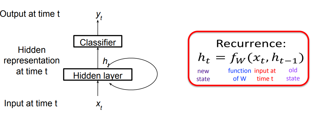
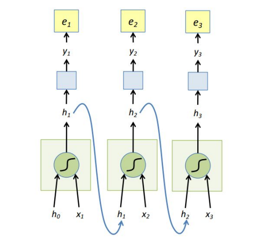
The hidden state $h_t$ is decided by $x_t$ and $h_{t-1}$ the hidden state at time $t-1$, $f_w$ injects non-linear weights into $x_t,h_{t-1}$. Classifier usually is a non-linear operation using softmax, assuming the output $y_t$ represents a probability: $$ h_t=tanh(W_x x_t + W_h h_{t-1}) \\ y_t = softmax(W_y h_t) $$ The unfolded graph provides an explicit description of which computations to perform:
.png)
RNNs are typically trained using backpropagation through time (BPTT), the unfolded network is treated as one big feed-forward network that accepts the whole time series as input. The weight updates are computed for each copy in the unfolded network, then summed or averaged and applied to the RNN weights. Here the loss function we use is cross entroy, and $y_{t_i}$ is the prediction of class $i, i=1,2,...,n$ (assume that we $n$ classes, the dimention of vector $y_t$ is $n \times 1$). $$ E(y,\hat y) = \sum_t E(y_t,\hat y_t) \\ E(y_t,\hat y_t) = - \sum_i \hat y_{t_i} log y_{t_i}\\ \frac{\partial e_3}{\partial W_y}=\frac{\partial e_3}{\partial y_3} \frac{\partial y_3}{\partial W_y}=(\hat y_3 -y_3) \otimes h_3 $$ $\otimes$ is outer product. $$ \begin{aligned} h_t&=tanh(W_x x_t + W_h h_{t-1})\\ \frac{\partial e_3}{\partial W_h} &= \frac{\partial e_3}{\partial y_3} \frac{\partial y_3}{\partial h_3}\frac{\partial h_3}{\partial W_h} \\&=\sum_{k=1}^3 \frac{\partial e_3}{\partial y_3} \frac{\partial y_3}{\partial h_3}\frac{\partial h_3}{\partial h_k}\frac{\partial h_k}{\partial W_h} \end{aligned} $$ The weights $W_h$ are shared and the partial derivative of $e_3$ with respect to $W_h$ is contributed by $h_1,h_2,h_3$. If input sequences are comprised of thousands of timesteps, then the same amount of derivatives required for a single update weight update. This can cause weights to vanish or explode, thus poor model performance. BPTT can be computationally expensive as the number of timesteps increases, as a result, we use truncated BPTT instead: 1. Present a sequence of k1 timesteps of input and output pairs to the network. 2. Unroll the network then calculate and accumulate errors across k2 timesteps. 3. Roll-up the network and update weights. 4. Repeat.
Most frequently used RNNs such as LSTM and GRU are not displayed here.
Transformer
CLICK ME
In recent years, transformers has shown it power in natural language process. Applications like Google translate, ChatGPT are based on the transformer architecture, which uses self-attention mechanism to process sequencial data in parallel and catch long-range dependency.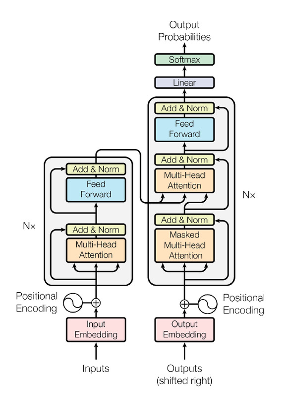
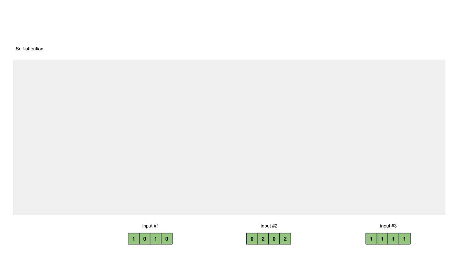
RNN has poor parallel capabilities and easily forgets long-distance information, but self-attention overcomes these shortcomings. The attention mechanism allows the model to focus on specific parts of the input sequence and produce a weighted representation of the entire sequence, which can then be used for classification or prediction Let's see what happens to the input text. 1. Each input word is turned into a vector using an embedding algorithm; 2. Create 3 vectors from each input embedding(X), i.e. query(Q), key(K), value(V) by multiplying three matrices learned during the training process. $$ Q=XW^q,K=XW^k,V=XW^v $$ 3. Calculate a attention score for each word/embedding by scaled dot product of query and value matrix, and get the output value matrix of each word, which is then input to the next layer. $$ Score(Q,K)=\frac{QK^T}{\sqrt{d_k}} \\ Output_v(Q,K,V)=softmax(Score(Q,K))V $$ where Score(Q,K) is the attention score and Output_v(Q,K,V) is the output value of the attention layer, $d_k$ is the dimention of key vector. Specificly, the attention score of one word is calculated by sum all dot product between its query and all other key matrices, as displayed below (thanks to the author of this amazing gif):
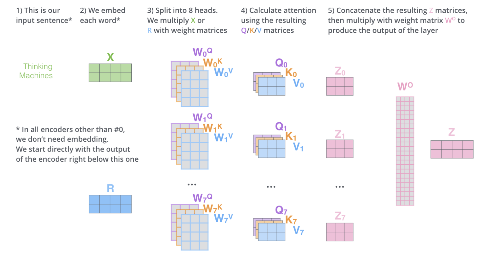
4. Each sub-layer (self-attention, ffnn) in each encoder has a residual connection around it, and is followed by layer-normalization step. 5. For the original transformer structure which is a encoder-decoder structure, the output of encoders is integrated into the decoder by encoder-decoder attention layer, decoder only structure (GPT) also works perfectly, which reveals the charm of self-attention mechanism. To capture more information in the input text, or gives the attention layer multiple “representation subspaces”, multi-head attention is normally used instead of plain self attention. In essence, we train multiple small weight matrices and concatenate the results into a big matrix. The calculation method of each result is the same as the calculation method of single-head attention. Finally, the generated b is connected to generate the final result. See the Img refered from: http://jalammar.github.io/illustrated-transformer/ . Another blog helps to understand the details of multi-head attention: https://hungsblog.de/en/technology/learnings/visual-explanation-of-multi-head-attention/
Masked Multi-head attention is to force the model to only see the sequence on its left and masks the sequence on its right, which prevent cheating while decoding. In practice, just add negative infinity to each value in the upper triangle part of attention score matrix (excluding diagonal), since softmax will naturally ignore small numbers. The transformer architecture also showed comparable performance to CNN in computer vision tasks after vision transformer (ViT) came out. More details will be added here after further research results appear.