Variational Autoencoder explained
Published:
Variational Autoencoders (VAEs) are a powerful class of generative models used in unsupervised learning, combining the strengths of both neural networks and probabilistic models. They aim to approximate an underlying latent space that represents the distribution of data. To achieve this, VAEs learn to encode high-dimensional input data into a lower dimensional set of latent variables using a variational inference process. By doing so, they can reconstruct the original input while also enabling manipulation and generation of new samples within the learned distribution. This is particularly useful for applications like image synthesis, where the ability to encode complex data and then decode it as new variations of that data is crucial.
Autoencoder
Autoencoder is an encoder-decoder structure nerual network, aims to learn a compressed representation of the data during encoding (also referred as feature extraction), and from which generate new data (reconstruct input) similar as possible to the original data. The formal definition [2]: Autoencoder is to learn the functions $A: R^n -> R^p$ (encoder) and $B: R^p -> R^n$ (decoder) that satisfy \(argmin_{A,B}E[\Delta (x,B A(x))],\) where $\Delta$ is the loss function that measures the distance between the output generated from the decoder and the input, $E$ is expectation, $B A(x)$ is the autoencoder output.
A generalization of PCA?
Note: In speaking of dimention reduction of data, one may think about Principal Component Analysis (PCA), which represent data using a low dimensional hyperplane (find a set of orthogonal basis). A linear autoencoder achieves the same result as PCA, but in practice we add non-linearity to encoder nerual network (also decoder), so the autoencoder learns a non-linear manifold instead.Variational Bayesian Inference
Basiclly, Bayesian Inference works in this way: first we choose a prior distribution over the unknown parameters or latent variables, then update it to a posterior distribution after seeing data. Variational Inference (VI) is an approach to obtain the posterior distribution by finding a surrogate distribution that approximates the true distribution. Another well-known way to calculate a posterior is MCMC, which tries to sample data from the posterior, usually computationally expensive(so slower than VI, but more accurate).
Bayesian Inference
Recall the Bayes' Rule: $$ p(b|a)=p(a|b)P(b)/p(a) $$ Assume $p(\theta)$ is a marginal distribution over model parameters $\theta$, i.e. a prior distribution. $p(D|\theta)$ is the According to the chain rule in probability, we have: $$ p(\theta,D)=p(\theta|D)p(D)=p(\theta)p(D|\theta) $$ Note that $p(D)$ is a constant, the posterior distribution over $\theta$ is: $$ p(\theta|D)=\frac{p(\theta)p(D|\theta)}{p(D)} \propto p(\theta)p(D|\theta) $$ That's the Bayes' Rule. $D$ here refers to the dataset consists of $n$ independently and identically distributed (i.i.d) observed datapoints ${x_1,x_2,...,x_n} \in D$. For convenience, $p(D|\theta)$, the likelihood of $D$ under model parameter $\theta$ (or the probability assigned to the data under the model with parameters $\theta$) is written as $p_\theta(D)$. We commonly use maximum log-likelihood to estimate $\theta$: $$ logp_\theta (D)=\sum_{x \in D}log p_\theta(x) $$ The aim is to search for a value of $\theta$ that makes $p_\theta(x)$ approaches to the true distribution $p^*(x)$. Then we can use Bayes' Rule to make prediction about new data $x_{new}$: $$ p(x=x_{new}|D)=\int p(x=x_{new},\theta|D)d\theta = \int p(x=x_{new}|\theta)p(\theta|D)d\theta $$In more complex cases, such as image generation, the model is parameterized with neural networks, and is not fully observed. We call such models deep latent variable model (DLVM), and variables that is not observed latent variables $z$ (e.g. encoded representation in autoencoders). We assume that the observed variables $x$ can be explained in terms of latent variables $z$: \(p_\theta(x)=\int p_\theta(x,z)dz=\int p_\theta(x|z)p(z)dz\) However, the marginal probability of data under the model $p_\theta(x)$ is intractable in DLVMs, since there’s no analytic solution or efficient estimator for the integral (hard to compute for high dimentional variables). Note that $p_\theta(x,z)$ is tractable and easy to compute. A tractable marginal likelihood $p_\theta(x)$ leads to a tractable posterior $p_\theta(z|x)$, and vice versa.
Variational inference approximates the $p_\theta(z|x)$ and $p_\theta(x)$ using parametrised distributions (e.g. Gaussian) by minimize an error (e.g. Kullback-Leibler divergence) between the approximation and target distribution. Now the inference is converted to an optimization problem. We find that minimizing the K-L divergence is equivalent to maximizing the ELBO (Evidence of Lower Bound), the derivation is given in the next section. One way to maximize ELBO is to assume independency between different dimentions of $z$ (mean-field theory) and proceed in a closed form optimization (coordinate ascent variational inference). While VAE takes another approach that is suitable for large dataset in deep neural networks, Stochastic Gradient Variational Bayes estimator, and you will see how it works in the next section as well.
From the perspective of functional analysis, both K-L divergence and ELBO are functional we want to find extreme points, find more below if you are interested in the mathematics.
Calculus of Variations
Variation is commonly used in finding the extreme value of a functional, e.g. finding a brachistochrone curve, or curve of fastest descent, which can be analogous to the derivation of ordinary functions. In mathematics, a functional is a special function that takes functions as input and output scalar numbers, a mapping from vector space to scalar domain (a function can be regarded as an infinite-dimensional vector). A simplest functional: $\int_a ^b f(x) dx$, input a function $f(x)$ and yield the area under the curve of $f(x)$ between $x=a$ and $x=b$. The output area depends on how $f(x)$, or the curve looks like. To put it in a more generalized way, a functional $I(y)$ can be like: $$ I(y)=\int_a ^b F(y,y';x)dx $$ Where $y,y'$ are functions of $x$, and here just write a first order derivative (there maybe higher order of derivatives). Usually $\delta$ is used to denote variation, e.g. $\delta y$ is the variation of $y(x)$, which means a tiny (infinitely small) change in $y(x)$ when $x$ remain unchanged. Note that $\delta y$ is caused by changes in the form of $y$, not $x$, since $dx$ here is supposed to be 0 (differ from derivative $dy$). The extreme value of $I(y)$ happens when $\delta I=0$, the same way we determine the extreme value of a function (the first order derivative of $\frac{df(x)}{dx}=0$, which could be explained in this way: near the extreme point, $f(x)$ remain unchanged when applying small changes to $x$). Introduce a differentiable function $h(x)$ as the increment of $y(x)$, $h(x)$ satisfies the boundary constraints $h(a)=h(b)=0$, $$ \begin{aligned} \delta I = I(y+h)-I(y) &= \int _a^b [F(y+h,y'+h';x)-F(y,y';x)]dx\\ &= \int _a^b [F_y(y,y';x)h+F_{y'}(y,y';x)h']dx +o(h^2) \\ &= \int _a^b [\frac{\partial F}{\partial y}-\frac{d}{dx}(\frac{\partial F}{\partial y'})]hdx+\frac{\partial F}{\partial y'}h |_{x=a}^{x=b}+o(h^2) \end{aligned} $$ the second line of the equation is derived by Taylor expansion of $F(y+h,y'+h';x)$, the third line is obtained using integration by parts. Since $\frac{\partial F}{\partial y'}h |_{x=a}^{x=b}=0$ and the hiher order term $o(h^2)$ is neglectable, if $\delta I=0$, the following equations exists: $$ \frac{\partial F}{\partial y}-\frac{d}{dx}(\frac{\partial F}{\partial y'})=0 $$ Yes, it's E-L equation.Variational Autoencoder
Let’s interpret VAE from a perspective of Bayesian inference. The encoder is an inference model $q_\phi (z|x)$ that obtains the compressed representation i.e. latent variables $z$ given observed variables $x$. The decoder $p_\theta (x|z)$ decode data from $z$ space back to $x$ space.
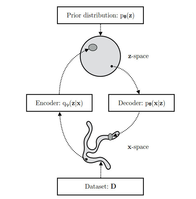
A VAE learns stochastic mappings between the observed x-space and a lantent z space. $\phi$ is the parameters of the encoder, and $\theta$ is the parameters of the decoder. $\theta$ is optimized to make the generated data more compatible with the distribution of real data; $\phi$ is optimized so that the encoder $q_\phi (z|x)$ approximates the true but intractable posterior $p_\theta (z|x)$ of the generative model.
\(q_\phi (z|x) \approx p_\theta (z|x)\)
We know that Kullback–Leibler divergence measures the distance of two distributions. Given two continuous distributions’ PDF $p(z)$, $q(z)$, the K-L divergence is defined as:
\(D_{KL}(q||p)=\int q(z)log(\frac{q(z)}{p(z)})dz\)
In practice, we choose evidence lower bound (ELBO) as the optimization objective of variational methods including VAE. See the following derivation.
\(\begin{aligned} logp_\theta(x)&=E_{q_\phi (z|x)}[logp_\theta(x)]\\ &=E_{q_\phi (z|x)}[log[\frac{p_\theta(x,z)}{p_\theta(z|x)}]]\\ &=E_{q_\phi (z|x)}[log[\frac{p_\theta(x,z)}{q_\phi (z|x)} \frac{q_\phi (z|x)}{p_\theta(z|x)}]]\\ &=E_{q_\phi (z|x)}[log[\frac{p_\theta(x,z)}{q_\phi (z|x)}]]+E_{q_\phi (z|x)}[log[\frac{q_\phi (z|x)}{p_\theta(z|x)}]] \\ &=L_{\theta,\phi}(x)+D_{KL}(q_\phi (z|x)||p_\theta (z|x)) \end{aligned}\)
From the equations above, we know that given a $p_\theta (x)$, maximizing ELBO is equivalent to minimizing K-L divergence, since the KL divergence between $q_\phi (z|x)$ and $p_\theta (z|x)$ is non-negative (equal to 0 if, and only if two distributions are equal).
\(\begin{aligned} L_{\theta,\phi}(x)&=logp_\theta(x)-D_{KL}(q_\phi (z|x)||p_\theta (z|x)) \\ &\leq logp_\theta(x) \end{aligned}\)
$L_{\theta,\phi}(x)$ is called variational lower bound, aka evidence lower bound (ELBO):
\(L_{\theta,\phi}(x)=E_{q_\phi (z|x)}[logp_\theta(x,z)-log q_\phi (z|x)]\)
We now see why choosing ELBO over KL divergence: in ELBO, we deal with the joint distribution $p_{\theta}(x,z)$ and posterior of inference model $q_\phi(z|x)$ ( which is tractable because we can choose the surrogate model), tactically avoid the intractable posterior $q_{\theta}(z|x)$ in generative model. Notably, maximizing ELBO w.r.t. $\theta$ and $\phi$ will not only minimize KL divergence of $q_\phi (z|x)$ from $p_\theta (z|x)$, but also maximize $p_\theta(x)$, which means both the inference model (encoder) and the generative model (decoder) get better.
The (unbiased) gradient of ELBO w.r.t. all parameters ($\phi$ and $\theta$) can be optimized using stochastic gradient descent (SGD). For $\theta$, we have:
\(\begin{aligned} \nabla_\theta L_{\theta,\phi}(x) &= \nabla_\theta E_{q_\phi (z|x)}[logp_\theta(x,z)-log q_\phi (z|x)]\\&=E_{q_\phi (z|x)}[\nabla_\theta(logp_\theta(x,z)-log q_\phi (z|x))]\\ & \simeq \nabla_\theta logp_\theta(x,z) \end{aligned}\)
So we can simply sample $z$ from $q_\phi (z|x)$ using Monte Carlo estimator. However, to get the gradient of ELBO w.r.t. $\phi$, we need a reparameterization trick that let $z$ be a function of $\phi,x$ and a random variable $\epsilon$. We cannot follow the same method as we did for $\theta$, because $q_\phi (z|x)$ is a function of $\phi$, the equation is not valid:
\(\begin{aligned} \nabla_\phi L_{\theta,\phi}(x) &= \nabla_\phi E_{q_\phi (z|x)}[logp_\theta(x,z)-log q_\phi (z|x)]\\& \neq E_{q_\phi (z|x)}[\nabla_\phi(logp_\theta(x,z)-log q_\phi (z|x))] \end{aligned}\)
After introducing $\epsilon$, the ELBO is rewritten as:
\(\begin{aligned} L_{\theta,\phi}(x) &= E_{q_\phi (z|x)}[logp_\theta(x,z)-log q_\phi (z|x)] \\ &= E_{p(\epsilon)}[logp_\theta(x,z)-log q_\phi (z|x)] \end{aligned}\)
where $z = g(\epsilon, \phi, x)$, and we can use Monte Carlo estimator to get $\nabla_\phi L_{\theta,\phi}(x)$ by sample random noise $\epsilon \sim p(\epsilon)$.
Reparameterization trick
Since we cannot compute gradients of the objective $f$ w.r.t. $\phi$ through the random variable $z \sim q_\phi (z|x)$, we can re-parameterizing $z$ as a deterministic and differentiable function of $\phi, x$, and a random variable $\epsilon$. In this way, we externalize the randomness in z by introducing $\epsilon$ (random noise) that is independent of $x$ or $phi$. We usually know the pdf of $p(\epsilon)$, e.g. we choose normal distribution for $\epsilon \sim N(0, I)$. $$ z = g(\epsilon, \phi, x) \\ E_{q_\phi (z|x)}[f(z)] = E_{p(\epsilon)}[f(z)] $$ Now we can use a simple Monte Carlo estimator to get the unbiased estimation of the gradients: $$ \begin{aligned} \nabla_\phi E_{q_\phi (z|x)}[f(z)] &= \nabla_\phi E_{p(\epsilon)}[f(z)] \\ &= E_{p(\epsilon)}[\nabla_\phi f(z)] \\ & \simeq \nabla_\phi f(z) \end{aligned} $$Reference:
[1] Kingma, Diederik Pieter. “Variational inference & deep learning: A new synthesis.” (2017).
[2] Bank, Dor, Noam Koenigstein, and Raja Giryes. “Autoencoders.” Machine learning for data science handbook: data mining and knowledge discovery handbook (2023): 353-374.
[3] Bishop, Christopher M., and Nasser M. Nasrabadi. Pattern recognition and machine learning. Vol. 4. No. 4. New York: springer, 2006.
[4] Calculus of Variations (https://courses.maths.ox.ac.uk/pluginfile.php/29848/mod_resource/content/1/Notes%202022.pdf)