Diffusion Probabilistic Models
Published:
Diffusion probabilistic models, or diffusion models for brevity are first proposed in [1]. The modified version called Denoising diffusion probabilistic models (DDPM) [2] were popularized due to the excellent high quality samples they generated, and Latent Diffusion Models (LDM) [3] make diffusion models practical.
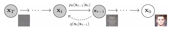
As a generative model, A DM models complex datasets in a computational tractable way [1]. Specificly, inspired by non-equilibrium statistical physics, a diffusion model first uses a parameterized Markov chain to gradually convert one distribution to another, usually gradually adds noise to the data to convert a very complex distribution to a simple one, e.g. normal distribution. Then it uses trainable Markov chain to reconstruct the target distribution from a simple known distribution.
Here an image $x_0 \sim q(x_0)$ is transitioned to an noisy image $x_t$ over $t$ timesteps by applying the Markov diffusion kernel $q(x_t|x_{t-1})$, or forward diffusion kernel. In the reverse process, $x_t$ is converted back to the target image $x_0$ by using the reverse diffusion kernel $p_\theta (x_t|x_{t-1})$, where $\theta$ represents trainable parameters.
Forward & Reverse Process
Forward Process
$$ q(x_1,x_2,...,x_T|x_0):=\prod \limits_{t=1}^T q(x_t|x_{t-1}) \\ q(x_t|x_{t-1}):= \mathcal N (x_t;\sqrt{1-\beta_t}x_{t-1},\beta_t I) $$ where $q(x_t|x_{t-1})$ is known as the forward diffusion kernel, $\beta _1,..., \beta _T$ is a variance schedule, which can be learned by reparameterization (refer to VAE) or held constant as hyperparameters. In the forward process or diffusion process, DDPM destroys the signal by gradually adding Gaussian noise to the data via a Markov chain and obtains the posterior $q(x_1,x_2,...,x_T|x_0)$ or $q(x_{1:T}|x_0)$ for simplicity, where the sampling chain transitions are set to conditional when the diffusion consists of small amounts of Gaussian noise. Thanks to the good traits of Gaussian distribution: Given N independent variables $r_1,...r_N$ that follow Gaussian distributions, the sum $\sum^N_{i=1} r_i$ still obeys Gaussian distribution. $$ r_i \sim \mathcal N(\mu_i,\sigma_i^2), i = 1,2,...,N \\ \sum^N_{i=1} r_i = \mathcal N(\sum^N_{i=1} \mu_i, \sum^N_{i=1} \sigma_i^2) $$ we can easily parameterize the neural network as shown below. The sample at timestep $t$: $$ x_t=\sqrt{1-\beta_t}x_{t-1} + \sqrt{\beta_t}\epsilon_{t-1} $$ where $\epsilon_{t-1} \sim \mathcal N(0,I)$, then let $\alpha_t = 1-\beta_t, \bar \alpha_t = \prod ^T _{i=1} \alpha_i$, substitute $\beta_t$: $$ \begin{aligned} x_t &= \sqrt{\alpha_t}x_{t-1}+\sqrt{1-\alpha_t}\epsilon_{t-1} \\ &= \sqrt{\alpha_t}(\sqrt{\alpha_{t-1}}x_{t-2}+\sqrt{1-\alpha_{t-1}}\epsilon_{t-2})+\sqrt{1-\alpha_t}\epsilon_{t-1} \ \ \ \ (\text{Expanding} \space x_{t-1})\\ &= \sqrt{\alpha_t \alpha_{t-1}}x_{t-2} + \sqrt{\alpha_t(1-\alpha_{t-1})}\epsilon_{t-2} + \sqrt{1-\alpha_t}\epsilon_{t-1} \\ &= \sqrt{\alpha_t \alpha_{t-1}}x_{t-2} + \sqrt{\alpha_t(1-\alpha_{t-1})+(1-\alpha_t)}\hat\epsilon \ \ \ \ (\text{Sum of Gaussian distributions})\\ &= \sqrt{\alpha_t \alpha_{t-1}}x_{t-2} + \sqrt{1-\alpha_t \alpha_{t-1}}\hat\epsilon\\ &= ...\\ &= \sqrt{\bar{\alpha_t}}x_0+\sqrt{1-\bar{\alpha_t}}\epsilon \end{aligned} $$ where $\epsilon \sim \mathcal N (0, I)$. Note that $\sqrt{\alpha_t(1-\alpha_{t-1})}\epsilon_{t-2} \sim \mathcal N (0, \alpha_t(1-\alpha_{t-1})), \sqrt{1-\alpha_t}\epsilon_{t-1} \sim \mathcal N (0, \sqrt{1-\alpha_t})$, the sum of these two Gaussians follows $\mathcal N (0,\sqrt{\alpha_t(1-\alpha_{t-1})+(1-\alpha_t)})$. The above derivations enable us to get samples from arbitary timestep directly without simulating the entire Markov chain, that is the charm of Gaussian distribution.Reverse Process
The reverse process starts from a standard Gaussian $p(x_T)=\mathcal N(x_T;0,I)$: $$ p_\theta (x_0,x_1,...,x_T):=p(x_T) \prod ^T_{t=1}p_\theta (x_{t-1}|x_t) \\ p_\theta (x_{t-1}|x_t) := \mathcal N(x_{t-1};\mu_\theta(x_t,t),\Sigma_\theta(x_t,t)) $$ The joint distribution $p(x_0,...,x_T)$ is called the reverse process and $p_\theta (x_{t-1}|x_t)$ is known as the reverse diffusion kernel. $\mu_\theta(x_t,t)$ and $\Sigma_\theta(x,t)$ are parameters learned by a neural network. The reverse process aims to remove the noise gradually using Markov chain to recover the original data.Objective Function
\(p_\theta (x_0) = \int p_\theta(x_0,x_1,...,x_T)dx_1dx_2...dx_T\) As a generative model, diffusion models are supposed to maximize the likelihood $p(x)$. However, integrating over all latent variables is intractable, we maximize Evidence Lower Bound (ELBO) instead.
Evidence Lower Bound
$$ E_{q_\phi (z|x)} [log \frac{p(x,z)}{q_\phi (z|x)}] $$ Here, $q_\phi(z|x)$ is a probabilistic model to estimate the true distribution over latent variables for given observations $x$. Two ways to derive ELBO, we can use Jensen's inequality: $$ \begin{aligned} \text{log }p(x)&=\text{log }\int p(x,z)dz \\ &=\text{log }\int \frac{p(x,z){q_\phi (z|x)}}dz\\ &=\text{log }E_{q_\phi (z|x)}[\frac{p(x,z)}{q_\phi (z|x)}]\\ &\geq E_{q_\phi (z|x)}[\text{log }\frac{p(x,z)}{q_\phi (z|x)}] \ \ \ \ \text{(Jensen's inequality)} \end{aligned} $$ or we can do it another way: $$ \begin{aligned} \text{log }p(x)&=\text{log }p(x) \underbrace{\int q_\phi(z|x) dz}_1 \\ &= \int q_\phi (z|x)(\text{log }p(x))dz \\ &= E_{q_\phi (z|x)}[\text{log }p(x)] \\ &= E_{q_\phi (z|x)}[\text{log } \frac{p(x,z)}{p(z|x)}] \\ &= E_{q_\phi (z|x)}[\text{log } \frac{p(x,z)q_\phi(z|x)}{p(z|x)q_\phi(z|x)}] \\ &= E_{q_\phi (z|x)}[\text{log } \frac{p(x,z)}{q_\phi (z|x)}]+\underbrace{E_{q_\phi (z|x)}[\text{log } \frac{q_\phi (z|x)}{p(z|x)}]}_{D_{KL}(q_\phi (z|x)||p(z|x))} \\ &\geq E_{q_\phi (z|x)}[\text{log } \frac{p(x,z)}{q_\phi (z|x)}] \ \ \ \ \ \ \text{(KL Divergence is non negative)} \end{aligned} $$ From the second derivation, we now clearly see that ELBO is indeed a lower bound. Moreover, maximizing ELBO is equavalent to minizing $D_{KL}(q_\phi (z|x)||p(z|x))$ considering that $p(x)$ is a constant w.r.t $\phi$, thus we are approaching the true latent posterior distribution as we optimize ELBO.In diffusion models, $x_0$ is observed data denoted by $x$, $x_1, x_2,…,x_T$ are hidden state denoted by $z$ in above ELBO derivations, and $q_\phi(z|x)$ is a Markov chain modeled by Gaussian distributions, so we can remove $\phi$ in later derivations. We can simply rewrite the ELBO as: \(\text{log } p(x) \geq E_{q(x_{1:T}|x_0)} [\text{log } \frac{p(x_{0:T})}{q(x_{1:T}|x_0)}]\) Take Markov property into consideration $q(x_t|x_{t-1})=q(x_t|x_{t-1},x_0)$, we continue this derivation: \(\begin{aligned} \text{log } p(x) &\geq E_{q(x_{1:T}|x_0)} [\text{log } \frac{p(x_{0:T})}{q(x_{1:T}|x_0)}]\\ &=E_{q(x_{1:T}|x_0)} [\text{log } \frac{p(x_T)\prod^T_{t=1}p_\theta(x_{t-1}|x_t)}{\prod^T_{t=1}q(x_t|x_{t-1})}]\\ &=E_{q(x_{1:T}|x_0)} [\text{log } \frac{p(x_T)p_\theta(x_0|x_1)\prod^T_{t=2}p_\theta(x_{t-1}|x_t)}{q(x_1|x_0)\prod^T_{t=2}q(x_t|x_{t-1},x_0)}]\\ &=E_{q(x_{1:T}|x_0)} [\text{log }\frac{p(x_T)p_\theta(x_0|x_1)}{q(x_1|x_0)}+\text{log } \prod^T_{t=2} \frac{p_\theta(x_{t-1}|x_t)}{\frac{q(x_{t-1}|x_t,x_0)q(x_t|x_0)}{q(x_{t-1}|x_0)}}] \ \ \ \ \ \text{(Bayes rule)}\\ &=E_{q(x_{1:T}|x_0)} [\text{log }\frac{p(x_T)p_\theta(x_0|x_1)}{q(x_1|x_0)}+\text{log }\frac{q(x_1|x_0)}{q(x_T|x_0)} +\text{log } \prod^T_{t=2} \frac{p_\theta(x_{t-1}|x_t)}{q(x_{t-1}|x_t,x_0)}] \\ &=E_{q(x_{1:T}|x_0)} [\text{log }\frac{p(x_T)p_\theta(x_0|x_1)}{q(x_T|x_0)}+\sum^T_{t=2}\text{log } \frac{p_\theta(x_{t-1}|x_t)}{q(x_{t-1}|x_t,x_0)}]\\ &=E_{q(x_{1:T}|x_0)}[\text{log }p_\theta(x_0|x_1)]+E_{q(x_{1:T}|x_0)}[\text{log }\frac{p(x_T)}{q(x_T|x_0)}]+\sum^T_{t=2}E_{q(x_{1:T}|x_0)}[\text{log } \frac{p_\theta(x_{t-1}|x_t)}{q(x_{t-1}|x_t,x_0)}] \\ &=E_{q(x_1|x_0)}[\text{log }p_\theta(x_0|x_1)]+E_{q(x_{T}|x_0)}[\text{log }\frac{p(x_T)}{q(x_T|x_0)}]+\sum^T_{t=2} \underbrace{E_{q(x_t,x_{t-1}|x_0)}[\text{log }\frac{p_\theta(x_{t-1}|x_t)}{q(x_{t-1}|x_t,x_0)}]}_{E_{q(x_t|x_0)}[E_{q(x_{t-1}|x_t,x_0)}\text{log }[\frac{p_\theta(x_{t-1}|x_t)}{q(x_{t-1}|x_t,x_0)}]]}\\ &=\underbrace{E_{q(x_1|x_0)}[\text{log }p_\theta(x_0|x_1)]}_{\text{RV1}}-\underbrace{D_{\text{KL}}(q(x_T|x_0)||p(x_T))}_{\text{RV2}}-\sum^T_{t=2} \underbrace{E_{q(x_t|x_0)}[D_{\text{KL}}(q(x_{t-1}|x_t,x_0)||p_\theta(x_{t-1}|x_t))]}_{\text{RV3}} \end{aligned}\)
The essence of this derivation is to use Bayes rule and Markov property, so we have the diffusion kernel written as:
\(q(x_t|x_{t-1},x_0)=\frac{q(x_{t-1}|x_t,x_0)q(x_t|x_0)}{q(x_{t-1}|x_0)}\)
Now look at the interpretation of ELBO, which consists of 3 terms:
a. RV1 is a reconstruction term, which can be optimized using a Monte Carlo estimate.
b. RV2 measures the distance between the distribution of the output of the forward process and the prior distribution of the reverse process. Since we assume that both are stardard Gaussian, RV2 is 0.
c. RV3 represents how close the distribution of learned denoising transition $ p_\theta(x_{t-1}|x_t) $ and the distribution of ground-truth denoising transition $ q(x_{t-1}|x_t,x_0) $ are. RV3 is called a denoising matching term, which we try to minimize so the learned denoising transition step is approaching the true distribution.
The optimization cost lies in the sum of RV3. Recall that for any timestep t, we have $x_t \sim \mathcal N(x_t;\sqrt{\bar \alpha_t}x_0,(1-\bar \alpha_t)I)$, and according to Bayes rule we have:
\(\begin{aligned} q(x_{t-1}|x_t,x_0)&=\frac{q(x_t|x_{t-1},x_0)q(x_{t-1}|x_0)}{q(x_t|x_0)}\\ &=\frac{\mathcal N(x_t;\sqrt{\alpha_t}x_{t-1},(1- \alpha_t)I) \ \mathcal N(x_{t-1};\sqrt{\bar \alpha_{t-1}}x_0,(1-\bar \alpha_{t-1})I)}{\mathcal N(x_t;\sqrt{\bar \alpha_t}x_0,(1-\bar \alpha_t)I)}\\ &\propto\text{exp} \left\{-[\frac{(x_t-\sqrt{\alpha_t}x_{t-1})^2}{2(1-\alpha_t)}+\frac{(x_{t-1}-\sqrt{\bar \alpha_{t-1}}x_0)^2}{2(1-\bar \alpha_{t-1})}-\frac{(x_t-\sqrt{\bar \alpha_t}x_0)^2}{2(1-\bar \alpha_t)}]\right\} \\ &=\text{exp} \left\{-\frac{1}{2}[\frac{-2\sqrt{\alpha_t}x_tx_{t-1}+\alpha_t x_{t-1}^2}{1-\alpha_t}+\frac{x_{t-1}^2-2\sqrt{\bar \alpha_{t-1}}x_{t-1}x_0}{1-\bar \alpha_{t-1}}+\underbrace{\frac{x_t^2}{1-\alpha_t}+\frac{\bar \alpha_{t-1}x_0^2}{1-\bar \alpha_{t-1}}-\frac{(x_t-\sqrt{\bar \alpha_t}x_0)^2}{1-\bar \alpha_t}}_{C(x_t,x_0)}]\right\} \\ &=\text{exp} \left\{-\frac{1}{2}[(\frac{\alpha_t}{1-\alpha_t}+\frac{1}{1-\bar \alpha_{t-1}})x_{t-1}^2-2(\frac{\sqrt{\alpha_t}x_t}{1-\alpha_t}+\frac{\sqrt{\bar \alpha_{t-1}}x_0}{1-\bar \alpha_{t-1}})x_{t-1}+C(x_t,x_0)]\right\}\\ &=\text{exp} \left\{- \frac{1-\bar \alpha_t}{2(1- \alpha_t)(1-\bar \alpha_{t-1})}[x_{t-1}^2-2\frac{\sqrt{\alpha_t}(1-\bar \alpha_{t-1})x_t+\sqrt{\bar \alpha_{t-1}}(1-\alpha_t)x_0}{1-\bar \alpha_t}x_{t-1}+\frac{\alpha_t(1-\bar\alpha_{t-1})^2x_t^2+\bar\alpha_{t-1}(1-\alpha_t)^2x_0^2+2\sqrt{\bar \alpha_t}(1-\alpha_t)(1-\bar \alpha_{t-1})x_tx_0}{(1-\bar \alpha_t)^2}]\right\}\\ &=\text{exp} \left\{ -\frac{1}{2 \cdot \frac{(1- \alpha_t)(1-\bar \alpha_{t-1})}{1-\bar \alpha_t}}(x_{t-1}-\frac{\sqrt{\alpha_t}(1-\bar \alpha_{t-1})x_t+\sqrt{\bar \alpha_{t-1}}(1-\alpha_t)x_0}{1-\bar \alpha_t})^2 \right\}\\ &=\mathcal N(x_{t-1};\underbrace{\frac{\sqrt{\alpha_t}(1-\bar \alpha_{t-1})x_t+\sqrt{\bar \alpha_{t-1}}(1-\alpha_t)x_0}{1-\bar \alpha_t}}_{\mu_q(x_t,x_0)},\underbrace{\frac{(1- \alpha_t)(1-\bar \alpha_{t-1})}{1-\bar \alpha_t}I}_{\Sigma_q(t)}) \end{aligned}\) Note that $\alpha$ coefficients are known and frozen at each timestep, in order for $p_\theta(x_{t-1}|x_t)$ to approach $q(x_{t-1}|x_t,x_0)$, we can construct its varience $\Sigma_\theta=\Sigma_q$ and mean $\mu_\theta$ as a function of $x_t$. The mean of $q(x_{t-1}|x_t,x_0)$:
\(\mu_q(x_t,x_0)=\frac{\sqrt{\alpha_t}(1-\bar \alpha_{t-1})x_t+\sqrt{\bar \alpha_{t-1}}(1-\alpha_t)x_0}{1-\bar \alpha_t}\)
Follow the form of $\mu_q$, we have:
\(\mu_\theta(x_t,x_0)=\frac{\sqrt{\alpha_t}(1-\bar \alpha_{t-1})x_t+\sqrt{\bar \alpha_{t-1}}(1-\alpha_t) \hat x_\theta(x_t,t)}{1-\bar \alpha_t}\)
where $\hat x_\theta(x_t,t)$ is the prediction of original data $x_0$ from noisy data $x_t$ at timestep $t$.
KL Divergence between two Gaussian distributions
The $D_\text{KL}$ between two Gaussians is: $$ D_{\text{KL}}(\mathcal N(x;\mu_x,\Sigma_x)||\mathcal N(y;\mu_y,\Sigma_y))=\frac{1}{2}[\text{log}\frac{|\Sigma_y|}{|\Sigma_x|}-d+\text{tr}(\Sigma_y^{-1}\Sigma_x)+(\mu_y-\mu_x)^T\Sigma_y^{-1}(\mu_y-\mu_x)] $$Our goal is to minimize the KL Divergence:
\(\begin{aligned} L &=\underset{\theta}{\text{arg min }} D_{\text{KL}}(q(x_{t-1}|x_t,x_0)||p_\theta(x_{t-1}|x_t))\\ &=\underset{\theta}{\text{arg min }} D_{\text{KL}}(\mathcal N(x_{t-1};\mu_q,\Sigma_q(t))||\mathcal N(x_{t-1};\mu_\theta,\Sigma_q(t)))\\ &=\underset{\theta}{\text{arg min }} \frac{1}{2}[(\mu_\theta-\mu_q)^T\Sigma_q(t)^{-1}(\mu_\theta-\mu_q)]\\ &=\underset{\theta}{\text{arg min }} \frac{1}{2\sigma_q^2(t)}[||\mu_\theta-\mu_q||_2^2] \end{aligned}\)
Here we rewrite $\Sigma_q(t)=\sigma_q^2(t)$. Substitute $\mu_q$, $\mu_\theta$:
\(\begin{aligned} L &=\underset{\theta}{\text{arg min }} \frac{1}{2\sigma_q^2(t)}[||\frac{\sqrt{\bar \alpha_{t-1}}(1-\alpha_t)}{1-\bar \alpha_t}(\hat x_\theta(x_t,t)-x_0)||^2_2]\\ &=\underset{\theta}{\text{arg min }}\frac{\bar \alpha_{t-1}(1-\alpha_t)^2}{2\sigma_q^2(t)(1-\bar \alpha_t)^2}[||\hat x_\theta(x_t,t)-x_0||^2_2] \end{aligned}\)
In this way, a neural network is trained to predict the original data $x_0$ from a noisy data $x_t$ at any timestep $t$. While DDPM in [2] take a step further, write $x_0$ using reparameterization as:
\(x_0 = \frac{x_t-\sqrt{1-\bar \alpha_t}\epsilon_0}{\sqrt{\bar \alpha_t}}\)
Bring this into $\mu_q$:
\(\begin{aligned} \mu_q(x_t,x_0)&=\frac{\sqrt{\alpha_t}(1-\bar \alpha_{t-1})x_t+\sqrt{\bar \alpha_{t-1}}(1-\alpha_t)x_0}{1-\bar \alpha_t}\\ &=\frac{\sqrt{\alpha_t}(1-\bar \alpha_{t-1})x_t+(1-\alpha_t)\frac{x_t-\sqrt{1-\bar \alpha_t}\epsilon_0}{\sqrt{\alpha_t}}}{1-\bar \alpha_t}\\ &=(\frac{\sqrt{\alpha_t}(1-\bar \alpha_{t-1})}{1-\bar \alpha_t}+\frac{1-\alpha_t}{(1-\bar \alpha_t)\sqrt{\alpha_t}})x_t - \frac{(1-\alpha_t)\sqrt{1-\bar \alpha_t}}{(1-\bar \alpha_t)\sqrt{\alpha_t}}\epsilon_0 \\ &=\frac{1}{\sqrt{\alpha_t}}x_t - \frac{1-\alpha_t}{\sqrt{1-\bar \alpha_t}\sqrt{\alpha_t}}\epsilon_0 \end{aligned}\)
Accordingly we set $\mu_\theta$ as:
\(\mu_\theta (x_t,t)=\frac{1}{\sqrt{\alpha_t}}x_t - \frac{1-\alpha_t}{\sqrt{1-\bar \alpha_t}\sqrt{\alpha_t}}\hat \epsilon_\theta(x_t,t)\)
and plug this into our optimization problem:
\(\begin{aligned} L&=\underset{\theta}{\text{arg min }} D_{\text{KL}}(q(x_{t-1}|x_t,x_0)||p_\theta(x_{t-1}|x_t))\\ &=\underset{\theta}{\text{arg min }} D_{\text{KL}}(\mathcal N(x_{t-1};\mu_q,\Sigma_q(t))||\mathcal N(x_{t-1};\mu_\theta,\Sigma_q(t)))\\ &=\underset{\theta}{\text{arg min }} \frac{1}{2\sigma_q^2(t)}[||\mu_\theta-\mu_q||_2^2]\\ &=\underset{\theta}{\text{arg min }} \frac{1}{2\sigma_q^2(t)}[||\frac{1}{\sqrt{\alpha_t}}x_t - \frac{1-\alpha_t}{\sqrt{1-\bar \alpha_t}\sqrt{\alpha_t}}\hat \epsilon_\theta(x_t,t)-\frac{1}{\sqrt{\alpha_t}}x_t + \frac{1-\alpha_t}{\sqrt{1-\bar \alpha_t}\sqrt{\alpha_t}}\epsilon_0||_2^2]\\ &=\underset{\theta}{\text{arg min }} \frac{1}{2\sigma_q^2(t)}[||\frac{1-\alpha_t}{\sqrt{1-\bar \alpha_t}\sqrt{\alpha_t}}(\epsilon_0-\hat \epsilon_\theta(x_t,t))||_2^2]\\ &=\underset{\theta}{\text{arg min }} \frac{1}{2\sigma_q^2(t)}\frac{(1-\alpha_t)^2}{(1-\bar \alpha_t)\alpha_t}[||\epsilon_0-\hat \epsilon_\theta(x_t,t)||_2^2] \end{aligned}\)
Here a neural network $\hat \epsilon_\theta(x_t,t)$ is learned to predict $\epsilon_0 \sim \mathcal N(\epsilon;0,1)$. Mathematically learning noise is equivalent to learning the original data, but in practice, DDPM [2], which learns to predict noise, achieves better performance.
There’s another equivalent interpretations related to score-based generative models, refers to [5] for more info.
From VAE to DM
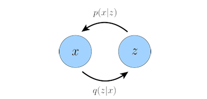
This section gives some background knowledge for readers to better understand VAE and diffusion models, and relationship between the two popular types of generative models. Let’s start from VAE, for more detailed illustration please read VAE. A Variational Autoencoder follows a simple encoder-decoder structure, encoder $q(z|x)$ learns the distribution over latent variables $z$ given observations $x$, decoder $p(x|z)$ generates data in observation space from the latent variables:
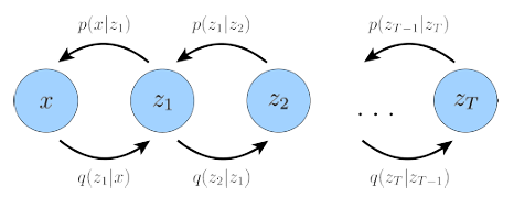
A generalization of a VAE called Hierarchical Variational Autoencoder (HVAE)extends latent variables to multiple hierarchies. If each transition down the hierarchy is Markovian, we call it a Markovian HVAE (MHVAE), which seems to be a stack of VAEs:
A Diffusion Model is also a special MHVAE, but its encoder is pre-defined as a linear Gaussian model and at final timestep the distribution of the latent is a standard Gaussian. The latent dimension is equal to the data dimension, while some improvements are made using Perceptual Compression to speed up both training and inference process [3].
Reference:
[1] Sohl-Dickstein, Jascha, et al. “Deep unsupervised learning using nonequilibrium thermodynamics.” International conference on machine learning. PMLR, 2015.
[2] Ho, Jonathan, Ajay Jain, and Pieter Abbeel. “Denoising diffusion probabilistic models.” Advances in neural information processing systems 33 (2020): 6840-6851.
[3] Rombach, Robin, et al. “High-resolution image synthesis with latent diffusion models.” Proceedings of the IEEE/CVF conference on computer vision and pattern recognition. 2022.
[4] Nichol, Alexander Quinn, and Prafulla Dhariwal. “Improved denoising diffusion probabilistic models.” International conference on machine learning. PMLR, 2021.
[5] Luo, Calvin. “Understanding diffusion models: A unified perspective.” arXiv preprint arXiv:2208.11970 (2022).