Large Language Models (LLMs) have revolutionized the field of natural language processing, enabling significant advancements in tasks such as language translation, text summarization, and sentiment analysis. However, despite their impressive capabilities, LLMs are not without limitations. One of the most significant challenges facing LLMs today is the problem of inference speed. Due to the sheer size and complexity of these models, the process of making predictions or extracting information from them can be computationally expensive and time-consuming. Several ways to speed up the LLMs without updating hardware:
a. Parallelism: Transformers are designed to work in parallel (Self-attention). One can take advantage of parallel processing on multi-core CPUs or multi-GPU systems.
b. Quantization: Quantizing the weights and activations of neural networks can help reduce the computational requirements for inference, meanwhile save memory usage.
c. Pruning: Pruning techniques can be used to remove redundant connections in neural networks, thereby reducing their size and computational requirements.
d. Knowledge Distillation: This technique involves transferring knowledge from a larger pre-trained model (the teacher) to a smaller model (the student). By leveraging the knowledge learned by the teacher, the student model can achieve better performance with less computational resources.
There are simplier ways, from engineering perspective, to optimizae LLM inference without changing the model architecture: 1. Reduce duplicate calculations (fewer FLOPs), 2. Reduce data transfer time (flash attention)
KV Cache
During inference, an LLM produces its output token by token, also known as autoregressive decoding. Each generated token depends on all previous tokens, including those in the prompt and any previously generated output tokens.
Therefore, the Key and Value of previous tokens are involved in the computation for the next token. The long queue of tokens can cause computation bottleneck in the self-attention stage, if we don’t use the K, V calculated before. To better illustrate this issue, here’s an example shows how self attention works.
The attention score of the first token is obtained by: \(Att_1(Q,K,V)=softmax(\frac{Q_1K^T_1}{\sqrt{d}})\vec{V_1}\) where $K=W_k x$, $Q=W_q x$, $V=W_v x$, $x$ is embedding vector, $d$ is the dimension of embedding vectors, we can overlook it in this discussion. When generating the second token, attention matrix: \(\begin{aligned} Att(Q,K,V) &=softmax( \begin{bmatrix} Q_1K^T_1 & - \infty \\ Q_2K^T_1 & Q_2K^T_2 \end{bmatrix} ) \begin{bmatrix} \vec{V_1} \\ \vec{V_2} \end{bmatrix} \\ &= \begin{bmatrix} softmax(Q_1K^T_1)\vec{V_1} \\ softmax(Q_2K^T_1)\vec{V_1} + softmax(Q_2K^T_2)\vec{V_2} \end{bmatrix} \end{aligned}\) Attention score for the second token is: \(Att_2(Q,K,V)=softmax(Q_2K^T_1)\vec{V_1} + softmax(Q_2K^T_2)\vec{V_2}\) Likewise, we can get the attention score for the thrid token: \(Att_3(Q,K,V)=softmax(Q_3K^T_1)\vec{V_1} + softmax(Q_3K^T_2)\vec{V_2} + softmax(Q_3K^T_3)\vec{V_3}\) We can see Key and Value used from last iteration are reused to generate the next token, thus store K, V to reduce computation.
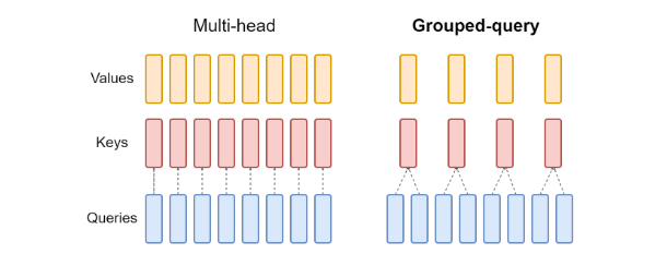
Memory is eaten up? KV cache can be very large, sometimes up to several GB. Let's see its size if data is stored in fp16 (2 bytes) for a single batch: $$ kv_size = 2*2*d*n_layers * max_context_length $$ Note that for Grouped-query Attention (GQA), multiple heads shared the same Key and Value, which could reduce the kv cache size. There are research ongoing showing that quantized (with some tricks) KV cache also works as well, things aren't that bad. Overall, more memory consumption for less computation and faster inference, it's a fair trade-off.
PagedAttention
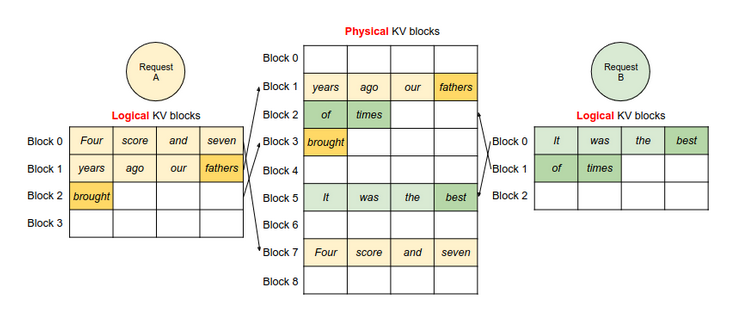
In the begining, KV cache is simply saved in VRAM, which requires large contiguous memory allocation. PagedAttention finds that there’s a considerable amount of memory being wasted in the KV cache because of excessive reservation. Instead of directly allocate the maximum amount of memory to fill the model context length, no matter how long the real prompt and generation would be, Pagedattention dynamicly allocates memory and save KV cache in non-contiguous blocks:
Pagedattention allows more sophisticated management, for instance, when multiple inference requests share the same large initial system prompt, it’s wise to save key and value vectors for the initial prompt once and share among requests. Now you can tell why the Pagedattention is so popular: it increases model throughput without any architecture modification, functions as a cache management layer that can be seamlessly integrated with various LLMs, especially useful in scenarios where LLMs handle large batches of prompts.
Further thoughts on memory management, pre-allocating memory is not bad as long as the allocated blocks are filled. vAttension pre-reserves virtual memory (continuous) to save the time on looking up block tables in Pagedattention, and allocates physical memory in runtime – one page at a time and only when a request has used all of its previously allocated physical memory page.
Flash Attention
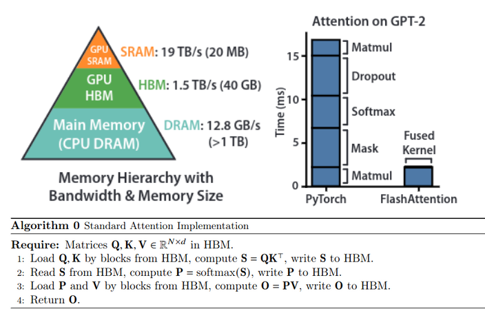
Authors of Flash attention found that attention operation is memory-bound caused by tensor transfer within a GPU, which means instead of targeting at matrix multiplication and reducing FLOPs, an IO-aware attention is the key to acceleration and overcome speed bottleneck. To better understand the intention of flash attention, here’s the structure of GPU memory, standard attention implementation and its time cost.
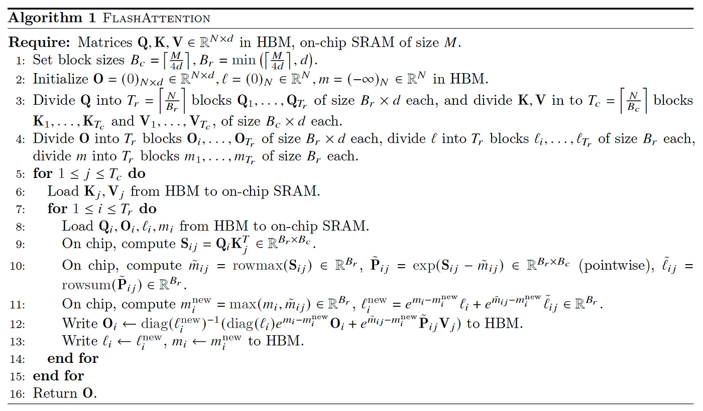
To perform a standard attention operation in GPU, tensors generated in intermediate steps are transfered between SRAM and HBM multiple times, results in much more time cost than matrix multiplication. In comparison, flash attention works in the following way:
The core is matrix split in softmax (also known as tiling). Recall the softmax computation of vector $x \in R^B$:
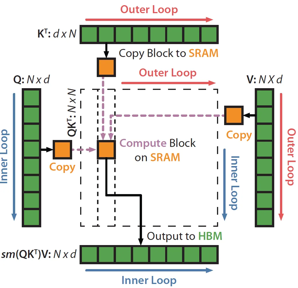
In this way, we can split $Q,K,V$ into blocks and incrementally perform the softmax reduction, compute softmax one block at a time. Flash attention does not store intermediate values ($S,P \in R^{N \times N}$ in algorithm 1) to compute gradients w.r.t $Q,K,V$ during backward pass, instead $S.P$ are recomputed by storing the output O and the softmax normalization statistics $(m,l)$. Recomputation not only reduces the required memory, but also speeds up the backward pass due to the reduction of HBM accesses. That’s why in algorithm 1 the block sizes are set to $\frac{M}{4d}$: blocks of $Q,K,V,O$ are loaded to SRAM and $m,l$ are kept in registers during computation. Another graph to illustrate:
The final road block when trying to understand algorithm 1 may lies in step 12. $O_i$ is intermediate computed attention result used during iteration. Since $S,P$ are not stored in memory, $\text{diag} (l_i) e^{m_i-m_i^{new}} O_i$ is to recover $PV$ from last iteration. Diagonal matrix here is a way to operate mul/div on matrix row by row, and the exponential part simply updates the new max value, these small mathematical tricks may be clearer after you verify it yourself. More details and proofs are provided in the paper.
Facilitated by the development of deep learning in subfields of computer vision including single object tracking (SOT), video object detection (VOD), and re-identification (Re-ID), many methods of multi-object tracking (MOT) have emerged, such as various embedding models designed for object locations and track identities [1]. While tracking-by-detection is still an effective paradigm for MOT, since we can always combine off-the-shelf state-of-the-art detectors and Re-ID models to improve the MOT system. The idea is: detect the objects in the current frame, then try to associate the detected boxes with tracked boxes in the previous frames. In practice, we need a more sophisticated design (e.g. choose similarity indices for data association, use Kalman Filter to predict new locations of tracks etc.) and proper strategies (e.g. to delete or initialize tracks). Hunarian algorithm is commonly used to matching objects after we get the similarity matrix, in this blog, I will try to explain how and why Hunarian algorithm works from the perspective of linear programming.
Problem Description
Hunarian algorithm or Kuhn-Munkres algorithm is well known for solving assignment problem, which involves assigning tasks to agents (or jobs to workers) such that the total cost is minimized (or the total profit is maximized), subject to the constraint that each agent is assigned exactly one task, and each task is assigned to exactly one agent.
Primal Form of the Assignment Problem
We are given an $n \times n$ cost matrix $C$, where $c_{ij}$ is the cost of assigning agent $i$ to task $j$. \(\begin{aligned} \text{min} & \sum_{i \in I} \sum_{j \in J} c_{ij}x_{ij} \\ s.t. & \sum_{j \in J}x_{ij} = 1 \text{ for all } i \in I \\ &\sum_{i \in I}x_{ij} = 1 \text{ for all } j \in J \\ & x_{ij} \geq 0 \end{aligned}\)
Note that $x_{ij} = 1$ if i is assigned to j and 0 otherwise.
Assignment Problem is a classic linear programming problem, since both the objective function and constraints are linear sums, even though it involves binary decision variables. We can model the problem as a bipartite graph and interpret the algorithm from the perspective of graph (find the perfect matching by finding augmenting path), but this blog will not cover this topic. Let’s try to understand Hungarian algorithm under the framework of linear programming. Since the primal problem is tricky to deal with, let’s go for the dual form of the problem.
Primal to Dual To convert the primal Assignment Problem to its dual form, we need to use Lagrange multipliers to relax the equality constraints in the primal problem. Introduce $u_i$ as the Lagrange multiplier associated with the constraint that agent $i$ is assigned exactly one task ($\sum_j x_{ij} = 1$), $v_j$ as the Lagrange multiplier associated with the constraint that task $j$ is assigned to exactly one agent ($\sum_i x_{ij} = 1$), then formulate the Lagrangian: $$ L(x_{ij},u_i,v_j)=\sum_{i=1}^n \sum_{j=1}^n c_{ij}x_{ij}+\sum_{i=1}^n u_i (1-\sum_{j=1}^n x_{ij})+\sum_{j=1}^n v_j (1-\sum_{i=1}^n x_{ij}) $$ Lagrange dual function is defined as the minimum value of the Lagrangian over primal variables: $$ g(u,v)=\text{inf}_x L(x,u,v) $$ where $\text{inf}_x$ means the infimum (the lower bound) of the Lagrangian over $x$. Since the dual function is the pointwise infimum of a family of affine functions of (u, ν), it is concave, even when the problem is not convex [2]. To minimize this Lagrangian $L(x_{ij},u_i,v_j)$ with respect to $x_{ij}$, rewrite the Lagrangian as: $$ L(x_{ij},u_i,v_j)=\sum_{i=1}^n \sum_{j=1}^n [(c_{ij}-u_i-v_j)x_{ij}] + \sum_{i=1}^n u_i + \sum_{j=1}^n v_j $$ The minimization occurs in the condition: $$ x_{ij}=1 \ \text{ if }\ c_{ij} \leq u_i+v_j \\ x_{ij}=0 \ \text{ if }\ c_{ij} > u_i+v_j $$ Now we want to find the tightest lower bound or minimum duality gap, so we need to maximize the dual function w.r.t $u$ and $v$. In the case of $x_{ij}=1$ If $c_{ij} \leq u_i+v_j$, the maximum occurs when $c_{ij} = u_i+v_j$, so $c_{ij}-u_i-v_j$ in Lagrangian is non-negative.
Dual Form of the Assignment Problem
The dual form of the Assignment Problem can be written as: \(\begin{aligned} \text{max} &\sum_{i=1}^n u_i + \sum_{j=1}^n v_j \\ s.t. & u_i+v_j \leq c_{ij}, \ \forall i, j \end{aligned}\)
where $u_i$ is the dual variable associated with agent $i$’s assignment constraint, $v_j$ is the dual variable associated with task $j$’s assignment constraint. The strong duality theorem of linear programming guarantees that if a feasible and bounded solution exists for the primal linear problem, the dual linear problem is feasible (and bounded as well, by weak duality), with the same optimum value as the primal [3]. The primal problem has constraints that ensure every agent is assigned exactly one task, and every task is assigned exactly one agent, a feasible primal solution exists (since the problem is well-posed with the same number of agents and tasks).
Hungarian Algorithm
Given a $n \times n$ cost matrix (Adjacent Matrix in Graph theory) $C$, the algorithm is summarized as 5 steps below:
Find and subtract the row minimum, namely find the minimum element in each row of the cost matrix and subtract the minimum element in each row from the element in that row.
Find and subtract the colume minimum, namely find the minimum element of each column in the remaining matrix and subtract the minimum element in each column from the elements in that column.
Use the minimum number of horizontal or vertical lines to cover all zero elements in the matrix. If the minimum number of lines is equal to $n$, stop running; if the minimum number of lines is less than $n$, continue to the next step.
Find the minimum value among the uncovered elements, subtract this minimum value from the uncovered elements, and add this minimum value to the elements at the intersection of different lines.
Go back to step 3, that is, continue to cover all zero elements in the matrix with the minimum number of horizontal or vertical lines. If the minimum number of lines is equal to $n$, stop running; if the minimum number of lines is less than $n$, execute step 4.
For details of $O(n^3)$ algorithm implementation, refer to this blog from cp algorithms, where the dual variables $u,v$ are denoted as potential. Hungarian algorithm updates the search of optimal value by continuesly increase the sum of $u,v$: \(f= \sum_{i=1}^n u[i] + \sum_{j=1}^n v[j]\)
In the context of MOT, cost matrix is filled with IOU or similarity score obtained from ReID features between objects in two consecutive frames. Sometimes the matrix is non-square, we can add dummy rows or columes with zeros and run more iterations.
Reference: [1] Wang, G., Song, M., & Hwang, J. N. (2022). Recent advances in embedding methods for multi-object tracking: a survey. arXiv preprint arXiv:2205.10766. [2] Boyd, Stephen, and Lieven Vandenberghe. Convex optimization. Cambridge university press, 2004. [3] Matoušek, Jiří, and Bernd Gärtner. Understanding and using linear programming. Vol. 1. Berlin: Springer, 2007.
In this blog, I’m going to share how I deployed LLMs (1~3b) and ASR models (whisper tiny & base) on my old smart phone, Xiaomi 8 (dipper). It was released in 2018, with a broken screen and depleted battery after several years of heavy usage, it still offers acceptable speed and fluency running daily light-weight apps. So I wonder, if I deploy modern machine models, such as LLMs, on the phone, and can I run the large models smoothly. Let’s see. The hardware configuration: 8-cores CPU with 4 big cores (Cortex-A75) and 4 small cores (Cortex-A55), 64 GB storage and 6 GB RAM. It has a integrated GPU, which I didn’t find a way to utilize during model inference, so the computation is totally counted on CPU in this trial. To better leverage the power of this CPU, I uninstall the android system (MIUI 12) and port a Ubuntu touch on the phone. Basically it’s a linux OS but using the underlying andriod framework to control hardwares, and it gives me a much longer battery life compared to android, also more convenience since I am a rookie in android development. Models are quantized versions from llamacpp and whispercpp. To get rid of the cumbersome work build an app with GUI, I run models in command line using the terminal app originally from Ubuntu touch, which can be regarded as the same terminal on Ubuntu desktop in this case. All I need to do is to compile the c++ code into an executable file that runs on my phone. Since the architecture of my laptop cpu is x86, the version of glibc, libstdc++ are different from the libs on the phone, I could either compile on the phone directly or cross compile on my PC with a specific toolchain. I kept all the heavy work on PC and built my own toolchain using crosstool-NG, which is targeted at building toolchains.
Large Language Models (LLMs) are the brains of various chatbots, and luckily we all have access to some brilliant cheap or even free LLMs now, thanks to open source community. It is possible to run LLMs on a PC and keep everything local. This blog presents my solution to building a chatbot running on my PC, with a totally local file storage system and a costumized graphical user interface.
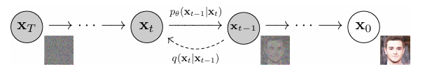
Diffusion probabilistic models, or diffusion models for brevity are first proposed in [1]. The modified version called Denoising diffusion probabilistic models (DDPM) [2] were popularized due to the excellent high quality samples they generated, and Latent Diffusion Models (LDM) [3] make diffusion models practical. As a generative model, A DM models complex datasets in a computational tractable way [1]. Specificly, inspired by non-equilibrium statistical physics, a diffusion model first uses a parameterized Markov chain to gradually convert one distribution to another, usually gradually adds noise to the data to convert a very complex distribution to a simple one, e.g. normal distribution. Then it uses trainable Markov chain to reconstruct the target distribution from a simple known distribution. Here an image $x_0 \sim q(x_0)$ is transitioned to an noisy image $x_t$ over $t$ timesteps by applying the Markov diffusion kernel $q(x_t|x_{t-1})$, or forward diffusion kernel. In the reverse process, $x_t$ is converted back to the target image $x_0$ by using the reverse diffusion kernel $p_\theta (x_t|x_{t-1})$, where $\theta$ represents trainable parameters.
Forward & Reverse Process
Forward Process $$ q(x_1,x_2,...,x_T|x_0):=\prod \limits_{t=1}^T q(x_t|x_{t-1}) \\ q(x_t|x_{t-1}):= \mathcal N (x_t;\sqrt{1-\beta_t}x_{t-1},\beta_t I) $$ where $q(x_t|x_{t-1})$ is known as the forward diffusion kernel, $\beta _1,..., \beta _T$ is a variance schedule, which can be learned by reparameterization (refer to VAE) or held constant as hyperparameters. In the forward process or diffusion process, DDPM destroys the signal by gradually adding Gaussian noise to the data via a Markov chain and obtains the posterior $q(x_1,x_2,...,x_T|x_0)$ or $q(x_{1:T}|x_0)$ for simplicity, where the sampling chain transitions are set to conditional when the diffusion consists of small amounts of Gaussian noise. Thanks to the good traits of Gaussian distribution: Given N independent variables $r_1,...r_N$ that follow Gaussian distributions, the sum $\sum^N_{i=1} r_i$ still obeys Gaussian distribution. $$ r_i \sim \mathcal N(\mu_i,\sigma_i^2), i = 1,2,...,N \\ \sum^N_{i=1} r_i = \mathcal N(\sum^N_{i=1} \mu_i, \sum^N_{i=1} \sigma_i^2) $$ we can easily parameterize the neural network as shown below. The sample at timestep $t$: $$ x_t=\sqrt{1-\beta_t}x_{t-1} + \sqrt{\beta_t}\epsilon_{t-1} $$ where $\epsilon_{t-1} \sim \mathcal N(0,I)$, then let $\alpha_t = 1-\beta_t, \bar \alpha_t = \prod ^T _{i=1} \alpha_i$, substitute $\beta_t$: $$ \begin{aligned} x_t &= \sqrt{\alpha_t}x_{t-1}+\sqrt{1-\alpha_t}\epsilon_{t-1} \\ &= \sqrt{\alpha_t}(\sqrt{\alpha_{t-1}}x_{t-2}+\sqrt{1-\alpha_{t-1}}\epsilon_{t-2})+\sqrt{1-\alpha_t}\epsilon_{t-1} \ \ \ \ (\text{Expanding} \space x_{t-1})\\ &= \sqrt{\alpha_t \alpha_{t-1}}x_{t-2} + \sqrt{\alpha_t(1-\alpha_{t-1})}\epsilon_{t-2} + \sqrt{1-\alpha_t}\epsilon_{t-1} \\ &= \sqrt{\alpha_t \alpha_{t-1}}x_{t-2} + \sqrt{\alpha_t(1-\alpha_{t-1})+(1-\alpha_t)}\hat\epsilon \ \ \ \ (\text{Sum of Gaussian distributions})\\ &= \sqrt{\alpha_t \alpha_{t-1}}x_{t-2} + \sqrt{1-\alpha_t \alpha_{t-1}}\hat\epsilon\\ &= ...\\ &= \sqrt{\bar{\alpha_t}}x_0+\sqrt{1-\bar{\alpha_t}}\epsilon \end{aligned} $$ where $\epsilon \sim \mathcal N (0, I)$. Note that $\sqrt{\alpha_t(1-\alpha_{t-1})}\epsilon_{t-2} \sim \mathcal N (0, \alpha_t(1-\alpha_{t-1})), \sqrt{1-\alpha_t}\epsilon_{t-1} \sim \mathcal N (0, \sqrt{1-\alpha_t})$, the sum of these two Gaussians follows $\mathcal N (0,\sqrt{\alpha_t(1-\alpha_{t-1})+(1-\alpha_t)})$. The above derivations enable us to get samples from arbitary timestep directly without simulating the entire Markov chain, that is the charm of Gaussian distribution.
Reverse Process The reverse process starts from a standard Gaussian $p(x_T)=\mathcal N(x_T;0,I)$: $$ p_\theta (x_0,x_1,...,x_T):=p(x_T) \prod ^T_{t=1}p_\theta (x_{t-1}|x_t) \\ p_\theta (x_{t-1}|x_t) := \mathcal N(x_{t-1};\mu_\theta(x_t,t),\Sigma_\theta(x_t,t)) $$ The joint distribution $p(x_0,...,x_T)$ is called the reverse process and $p_\theta (x_{t-1}|x_t)$ is known as the reverse diffusion kernel. $\mu_\theta(x_t,t)$ and $\Sigma_\theta(x,t)$ are parameters learned by a neural network. The reverse process aims to remove the noise gradually using Markov chain to recover the original data.
Objective Function
\(p_\theta (x_0) = \int p_\theta(x_0,x_1,...,x_T)dx_1dx_2...dx_T\) As a generative model, diffusion models are supposed to maximize the likelihood $p(x)$. However, integrating over all latent variables is intractable, we maximize Evidence Lower Bound (ELBO) instead.
Evidence Lower Bound $$ E_{q_\phi (z|x)} [log \frac{p(x,z)}{q_\phi (z|x)}] $$ Here, $q_\phi(z|x)$ is a probabilistic model to estimate the true distribution over latent variables for given observations $x$. Two ways to derive ELBO, we can use Jensen's inequality: $$ \begin{aligned} \text{log }p(x)&=\text{log }\int p(x,z)dz \\ &=\text{log }\int \frac{p(x,z){q_\phi (z|x)}}dz\\ &=\text{log }E_{q_\phi (z|x)}[\frac{p(x,z)}{q_\phi (z|x)}]\\ &\geq E_{q_\phi (z|x)}[\text{log }\frac{p(x,z)}{q_\phi (z|x)}] \ \ \ \ \text{(Jensen's inequality)} \end{aligned} $$ or we can do it another way: $$ \begin{aligned} \text{log }p(x)&=\text{log }p(x) \underbrace{\int q_\phi(z|x) dz}_1 \\ &= \int q_\phi (z|x)(\text{log }p(x))dz \\ &= E_{q_\phi (z|x)}[\text{log }p(x)] \\ &= E_{q_\phi (z|x)}[\text{log } \frac{p(x,z)}{p(z|x)}] \\ &= E_{q_\phi (z|x)}[\text{log } \frac{p(x,z)q_\phi(z|x)}{p(z|x)q_\phi(z|x)}] \\ &= E_{q_\phi (z|x)}[\text{log } \frac{p(x,z)}{q_\phi (z|x)}]+\underbrace{E_{q_\phi (z|x)}[\text{log } \frac{q_\phi (z|x)}{p(z|x)}]}_{D_{KL}(q_\phi (z|x)||p(z|x))} \\ &\geq E_{q_\phi (z|x)}[\text{log } \frac{p(x,z)}{q_\phi (z|x)}] \ \ \ \ \ \ \text{(KL Divergence is non negative)} \end{aligned} $$ From the second derivation, we now clearly see that ELBO is indeed a lower bound. Moreover, maximizing ELBO is equavalent to minizing $D_{KL}(q_\phi (z|x)||p(z|x))$ considering that $p(x)$ is a constant w.r.t $\phi$, thus we are approaching the true latent posterior distribution as we optimize ELBO.
In diffusion models, $x_0$ is observed data denoted by $x$, $x_1, x_2,…,x_T$ are hidden state denoted by $z$ in above ELBO derivations, and $q_\phi(z|x)$ is a Markov chain modeled by Gaussian distributions, so we can remove $\phi$ in later derivations. We can simply rewrite the ELBO as: \(\text{log } p(x) \geq E_{q(x_{1:T}|x_0)} [\text{log } \frac{p(x_{0:T})}{q(x_{1:T}|x_0)}]\) Take Markov property into consideration $q(x_t|x_{t-1})=q(x_t|x_{t-1},x_0)$, we continue this derivation: \(\begin{aligned} \text{log } p(x) &\geq E_{q(x_{1:T}|x_0)} [\text{log } \frac{p(x_{0:T})}{q(x_{1:T}|x_0)}]\\ &=E_{q(x_{1:T}|x_0)} [\text{log } \frac{p(x_T)\prod^T_{t=1}p_\theta(x_{t-1}|x_t)}{\prod^T_{t=1}q(x_t|x_{t-1})}]\\ &=E_{q(x_{1:T}|x_0)} [\text{log } \frac{p(x_T)p_\theta(x_0|x_1)\prod^T_{t=2}p_\theta(x_{t-1}|x_t)}{q(x_1|x_0)\prod^T_{t=2}q(x_t|x_{t-1},x_0)}]\\ &=E_{q(x_{1:T}|x_0)} [\text{log }\frac{p(x_T)p_\theta(x_0|x_1)}{q(x_1|x_0)}+\text{log } \prod^T_{t=2} \frac{p_\theta(x_{t-1}|x_t)}{\frac{q(x_{t-1}|x_t,x_0)q(x_t|x_0)}{q(x_{t-1}|x_0)}}] \ \ \ \ \ \text{(Bayes rule)}\\ &=E_{q(x_{1:T}|x_0)} [\text{log }\frac{p(x_T)p_\theta(x_0|x_1)}{q(x_1|x_0)}+\text{log }\frac{q(x_1|x_0)}{q(x_T|x_0)} +\text{log } \prod^T_{t=2} \frac{p_\theta(x_{t-1}|x_t)}{q(x_{t-1}|x_t,x_0)}] \\ &=E_{q(x_{1:T}|x_0)} [\text{log }\frac{p(x_T)p_\theta(x_0|x_1)}{q(x_T|x_0)}+\sum^T_{t=2}\text{log } \frac{p_\theta(x_{t-1}|x_t)}{q(x_{t-1}|x_t,x_0)}]\\ &=E_{q(x_{1:T}|x_0)}[\text{log }p_\theta(x_0|x_1)]+E_{q(x_{1:T}|x_0)}[\text{log }\frac{p(x_T)}{q(x_T|x_0)}]+\sum^T_{t=2}E_{q(x_{1:T}|x_0)}[\text{log } \frac{p_\theta(x_{t-1}|x_t)}{q(x_{t-1}|x_t,x_0)}] \\ &=E_{q(x_1|x_0)}[\text{log }p_\theta(x_0|x_1)]+E_{q(x_{T}|x_0)}[\text{log }\frac{p(x_T)}{q(x_T|x_0)}]+\sum^T_{t=2} \underbrace{E_{q(x_t,x_{t-1}|x_0)}[\text{log }\frac{p_\theta(x_{t-1}|x_t)}{q(x_{t-1}|x_t,x_0)}]}_{E_{q(x_t|x_0)}[E_{q(x_{t-1}|x_t,x_0)}\text{log }[\frac{p_\theta(x_{t-1}|x_t)}{q(x_{t-1}|x_t,x_0)}]]}\\ &=\underbrace{E_{q(x_1|x_0)}[\text{log }p_\theta(x_0|x_1)]}_{\text{RV1}}-\underbrace{D_{\text{KL}}(q(x_T|x_0)||p(x_T))}_{\text{RV2}}-\sum^T_{t=2} \underbrace{E_{q(x_t|x_0)}[D_{\text{KL}}(q(x_{t-1}|x_t,x_0)||p_\theta(x_{t-1}|x_t))]}_{\text{RV3}} \end{aligned}\)
The essence of this derivation is to use Bayes rule and Markov property, so we have the diffusion kernel written as: \(q(x_t|x_{t-1},x_0)=\frac{q(x_{t-1}|x_t,x_0)q(x_t|x_0)}{q(x_{t-1}|x_0)}\)
Now look at the interpretation of ELBO, which consists of 3 terms: a. RV1 is a reconstruction term, which can be optimized using a Monte Carlo estimate. b. RV2 measures the distance between the distribution of the output of the forward process and the prior distribution of the reverse process. Since we assume that both are stardard Gaussian, RV2 is 0. c. RV3 represents how close the distribution of learned denoising transition $ p_\theta(x_{t-1}|x_t) $ and the distribution of ground-truth denoising transition $ q(x_{t-1}|x_t,x_0) $ are. RV3 is called a denoising matching term, which we try to minimize so the learned denoising transition step is approaching the true distribution.
The optimization cost lies in the sum of RV3. Recall that for any timestep t, we have $x_t \sim \mathcal N(x_t;\sqrt{\bar \alpha_t}x_0,(1-\bar \alpha_t)I)$, and according to Bayes rule we have: \(\begin{aligned} q(x_{t-1}|x_t,x_0)&=\frac{q(x_t|x_{t-1},x_0)q(x_{t-1}|x_0)}{q(x_t|x_0)}\\ &=\frac{\mathcal N(x_t;\sqrt{\alpha_t}x_{t-1},(1- \alpha_t)I) \ \mathcal N(x_{t-1};\sqrt{\bar \alpha_{t-1}}x_0,(1-\bar \alpha_{t-1})I)}{\mathcal N(x_t;\sqrt{\bar \alpha_t}x_0,(1-\bar \alpha_t)I)}\\ &\propto\text{exp} \left\{-[\frac{(x_t-\sqrt{\alpha_t}x_{t-1})^2}{2(1-\alpha_t)}+\frac{(x_{t-1}-\sqrt{\bar \alpha_{t-1}}x_0)^2}{2(1-\bar \alpha_{t-1})}-\frac{(x_t-\sqrt{\bar \alpha_t}x_0)^2}{2(1-\bar \alpha_t)}]\right\} \\ &=\text{exp} \left\{-\frac{1}{2}[\frac{-2\sqrt{\alpha_t}x_tx_{t-1}+\alpha_t x_{t-1}^2}{1-\alpha_t}+\frac{x_{t-1}^2-2\sqrt{\bar \alpha_{t-1}}x_{t-1}x_0}{1-\bar \alpha_{t-1}}+\underbrace{\frac{x_t^2}{1-\alpha_t}+\frac{\bar \alpha_{t-1}x_0^2}{1-\bar \alpha_{t-1}}-\frac{(x_t-\sqrt{\bar \alpha_t}x_0)^2}{1-\bar \alpha_t}}_{C(x_t,x_0)}]\right\} \\ &=\text{exp} \left\{-\frac{1}{2}[(\frac{\alpha_t}{1-\alpha_t}+\frac{1}{1-\bar \alpha_{t-1}})x_{t-1}^2-2(\frac{\sqrt{\alpha_t}x_t}{1-\alpha_t}+\frac{\sqrt{\bar \alpha_{t-1}}x_0}{1-\bar \alpha_{t-1}})x_{t-1}+C(x_t,x_0)]\right\}\\ &=\text{exp} \left\{- \frac{1-\bar \alpha_t}{2(1- \alpha_t)(1-\bar \alpha_{t-1})}[x_{t-1}^2-2\frac{\sqrt{\alpha_t}(1-\bar \alpha_{t-1})x_t+\sqrt{\bar \alpha_{t-1}}(1-\alpha_t)x_0}{1-\bar \alpha_t}x_{t-1}+\frac{\alpha_t(1-\bar\alpha_{t-1})^2x_t^2+\bar\alpha_{t-1}(1-\alpha_t)^2x_0^2+2\sqrt{\bar \alpha_t}(1-\alpha_t)(1-\bar \alpha_{t-1})x_tx_0}{(1-\bar \alpha_t)^2}]\right\}\\ &=\text{exp} \left\{ -\frac{1}{2 \cdot \frac{(1- \alpha_t)(1-\bar \alpha_{t-1})}{1-\bar \alpha_t}}(x_{t-1}-\frac{\sqrt{\alpha_t}(1-\bar \alpha_{t-1})x_t+\sqrt{\bar \alpha_{t-1}}(1-\alpha_t)x_0}{1-\bar \alpha_t})^2 \right\}\\ &=\mathcal N(x_{t-1};\underbrace{\frac{\sqrt{\alpha_t}(1-\bar \alpha_{t-1})x_t+\sqrt{\bar \alpha_{t-1}}(1-\alpha_t)x_0}{1-\bar \alpha_t}}_{\mu_q(x_t,x_0)},\underbrace{\frac{(1- \alpha_t)(1-\bar \alpha_{t-1})}{1-\bar \alpha_t}I}_{\Sigma_q(t)}) \end{aligned}\) Note that $\alpha$ coefficients are known and frozen at each timestep, in order for $p_\theta(x_{t-1}|x_t)$ to approach $q(x_{t-1}|x_t,x_0)$, we can construct its varience $\Sigma_\theta=\Sigma_q$ and mean $\mu_\theta$ as a function of $x_t$. The mean of $q(x_{t-1}|x_t,x_0)$: \(\mu_q(x_t,x_0)=\frac{\sqrt{\alpha_t}(1-\bar \alpha_{t-1})x_t+\sqrt{\bar \alpha_{t-1}}(1-\alpha_t)x_0}{1-\bar \alpha_t}\)
Follow the form of $\mu_q$, we have: \(\mu_\theta(x_t,x_0)=\frac{\sqrt{\alpha_t}(1-\bar \alpha_{t-1})x_t+\sqrt{\bar \alpha_{t-1}}(1-\alpha_t) \hat x_\theta(x_t,t)}{1-\bar \alpha_t}\)
where $\hat x_\theta(x_t,t)$ is the prediction of original data $x_0$ from noisy data $x_t$ at timestep $t$.
KL Divergence between two Gaussian distributions The $D_\text{KL}$ between two Gaussians is: $$ D_{\text{KL}}(\mathcal N(x;\mu_x,\Sigma_x)||\mathcal N(y;\mu_y,\Sigma_y))=\frac{1}{2}[\text{log}\frac{|\Sigma_y|}{|\Sigma_x|}-d+\text{tr}(\Sigma_y^{-1}\Sigma_x)+(\mu_y-\mu_x)^T\Sigma_y^{-1}(\mu_y-\mu_x)] $$
Our goal is to minimize the KL Divergence: \(\begin{aligned} L &=\underset{\theta}{\text{arg min }} D_{\text{KL}}(q(x_{t-1}|x_t,x_0)||p_\theta(x_{t-1}|x_t))\\ &=\underset{\theta}{\text{arg min }} D_{\text{KL}}(\mathcal N(x_{t-1};\mu_q,\Sigma_q(t))||\mathcal N(x_{t-1};\mu_\theta,\Sigma_q(t)))\\ &=\underset{\theta}{\text{arg min }} \frac{1}{2}[(\mu_\theta-\mu_q)^T\Sigma_q(t)^{-1}(\mu_\theta-\mu_q)]\\ &=\underset{\theta}{\text{arg min }} \frac{1}{2\sigma_q^2(t)}[||\mu_\theta-\mu_q||_2^2] \end{aligned}\)
Here we rewrite $\Sigma_q(t)=\sigma_q^2(t)$. Substitute $\mu_q$, $\mu_\theta$: \(\begin{aligned} L &=\underset{\theta}{\text{arg min }} \frac{1}{2\sigma_q^2(t)}[||\frac{\sqrt{\bar \alpha_{t-1}}(1-\alpha_t)}{1-\bar \alpha_t}(\hat x_\theta(x_t,t)-x_0)||^2_2]\\ &=\underset{\theta}{\text{arg min }}\frac{\bar \alpha_{t-1}(1-\alpha_t)^2}{2\sigma_q^2(t)(1-\bar \alpha_t)^2}[||\hat x_\theta(x_t,t)-x_0||^2_2] \end{aligned}\)
In this way, a neural network is trained to predict the original data $x_0$ from a noisy data $x_t$ at any timestep $t$. While DDPM in [2] take a step further, write $x_0$ using reparameterization as: \(x_0 = \frac{x_t-\sqrt{1-\bar \alpha_t}\epsilon_0}{\sqrt{\bar \alpha_t}}\)
Accordingly we set $\mu_\theta$ as: \(\mu_\theta (x_t,t)=\frac{1}{\sqrt{\alpha_t}}x_t - \frac{1-\alpha_t}{\sqrt{1-\bar \alpha_t}\sqrt{\alpha_t}}\hat \epsilon_\theta(x_t,t)\)
and plug this into our optimization problem: \(\begin{aligned} L&=\underset{\theta}{\text{arg min }} D_{\text{KL}}(q(x_{t-1}|x_t,x_0)||p_\theta(x_{t-1}|x_t))\\ &=\underset{\theta}{\text{arg min }} D_{\text{KL}}(\mathcal N(x_{t-1};\mu_q,\Sigma_q(t))||\mathcal N(x_{t-1};\mu_\theta,\Sigma_q(t)))\\ &=\underset{\theta}{\text{arg min }} \frac{1}{2\sigma_q^2(t)}[||\mu_\theta-\mu_q||_2^2]\\ &=\underset{\theta}{\text{arg min }} \frac{1}{2\sigma_q^2(t)}[||\frac{1}{\sqrt{\alpha_t}}x_t - \frac{1-\alpha_t}{\sqrt{1-\bar \alpha_t}\sqrt{\alpha_t}}\hat \epsilon_\theta(x_t,t)-\frac{1}{\sqrt{\alpha_t}}x_t + \frac{1-\alpha_t}{\sqrt{1-\bar \alpha_t}\sqrt{\alpha_t}}\epsilon_0||_2^2]\\ &=\underset{\theta}{\text{arg min }} \frac{1}{2\sigma_q^2(t)}[||\frac{1-\alpha_t}{\sqrt{1-\bar \alpha_t}\sqrt{\alpha_t}}(\epsilon_0-\hat \epsilon_\theta(x_t,t))||_2^2]\\ &=\underset{\theta}{\text{arg min }} \frac{1}{2\sigma_q^2(t)}\frac{(1-\alpha_t)^2}{(1-\bar \alpha_t)\alpha_t}[||\epsilon_0-\hat \epsilon_\theta(x_t,t)||_2^2] \end{aligned}\)
Here a neural network $\hat \epsilon_\theta(x_t,t)$ is learned to predict $\epsilon_0 \sim \mathcal N(\epsilon;0,1)$. Mathematically learning noise is equivalent to learning the original data, but in practice, DDPM [2], which learns to predict noise, achieves better performance. There’s another equivalent interpretations related to score-based generative models, refers to [5] for more info.
From VAE to DM
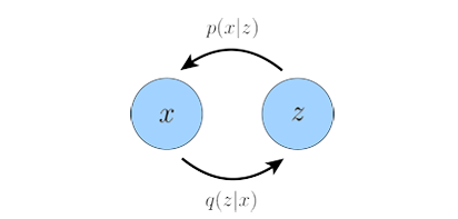
This section gives some background knowledge for readers to better understand VAE and diffusion models, and relationship between the two popular types of generative models. Let’s start from VAE, for more detailed illustration please read VAE. A Variational Autoencoder follows a simple encoder-decoder structure, encoder $q(z|x)$ learns the distribution over latent variables $z$ given observations $x$, decoder $p(x|z)$ generates data in observation space from the latent variables:
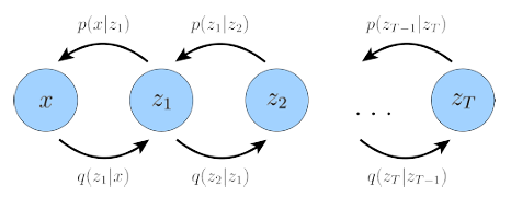
A generalization of a VAE called Hierarchical Variational Autoencoder (HVAE)extends latent variables to multiple hierarchies. If each transition down the hierarchy is Markovian, we call it a Markovian HVAE (MHVAE), which seems to be a stack of VAEs:
A Diffusion Model is also a special MHVAE, but its encoder is pre-defined as a linear Gaussian model and at final timestep the distribution of the latent is a standard Gaussian. The latent dimension is equal to the data dimension, while some improvements are made using Perceptual Compression to speed up both training and inference process [3].
Reference: [1] Sohl-Dickstein, Jascha, et al. “Deep unsupervised learning using nonequilibrium thermodynamics.” International conference on machine learning. PMLR, 2015. [2] Ho, Jonathan, Ajay Jain, and Pieter Abbeel. “Denoising diffusion probabilistic models.” Advances in neural information processing systems 33 (2020): 6840-6851. [3] Rombach, Robin, et al. “High-resolution image synthesis with latent diffusion models.” Proceedings of the IEEE/CVF conference on computer vision and pattern recognition. 2022. [4] Nichol, Alexander Quinn, and Prafulla Dhariwal. “Improved denoising diffusion probabilistic models.” International conference on machine learning. PMLR, 2021. [5] Luo, Calvin. “Understanding diffusion models: A unified perspective.” arXiv preprint arXiv:2208.11970 (2022).