Facilitated by the development of deep learning in subfields of computer vision including single object tracking (SOT), video object detection (VOD), and re-identification (Re-ID), many methods of multi-object tracking (MOT) have emerged, such as various embedding models designed for object locations and track identities [1]. While tracking-by-detection is still an effective paradigm for MOT, since we can always combine off-the-shelf state-of-the-art detectors and Re-ID models to improve the MOT system. The idea is: detect the objects in the current frame, then try to associate the detected boxes with tracked boxes in the previous frames. In practice, we need a more sophisticated design (e.g. choose similarity indices for data association, use Kalman Filter to predict new locations of tracks etc.) and proper strategies (e.g. to delete or initialize tracks). Hunarian algorithm is commonly used to matching objects after we get the similarity matrix, in this blog, I will try to explain how and why Hunarian algorithm works from the perspective of linear programming.
Problem Description
Hunarian algorithm or Kuhn-Munkres algorithm is well known for solving assignment problem, which involves assigning tasks to agents (or jobs to workers) such that the total cost is minimized (or the total profit is maximized), subject to the constraint that each agent is assigned exactly one task, and each task is assigned to exactly one agent.
Primal Form of the Assignment Problem
We are given an $n \times n$ cost matrix $C$, where $c_{ij}$ is the cost of assigning agent $i$ to task $j$. \(\begin{aligned} \text{min} & \sum_{i \in I} \sum_{j \in J} c_{ij}x_{ij} \\ s.t. & \sum_{j \in J}x_{ij} = 1 \text{ for all } i \in I \\ &\sum_{i \in I}x_{ij} = 1 \text{ for all } j \in J \\ & x_{ij} \geq 0 \end{aligned}\)
Note that $x_{ij} = 1$ if i is assigned to j and 0 otherwise.
Assignment Problem is a classic linear programming problem, since both the objective function and constraints are linear sums, even though it involves binary decision variables. We can model the problem as a bipartite graph and interpret the algorithm from the perspective of graph (find the perfect matching by finding augmenting path), but this blog will not cover this topic. Let’s try to understand Hungarian algorithm under the framework of linear programming. Since the primal problem is tricky to deal with, let’s go for the dual form of the problem.
Primal to Dual To convert the primal Assignment Problem to its dual form, we need to use Lagrange multipliers to relax the equality constraints in the primal problem. Introduce $u_i$ as the Lagrange multiplier associated with the constraint that agent $i$ is assigned exactly one task ($\sum_j x_{ij} = 1$), $v_j$ as the Lagrange multiplier associated with the constraint that task $j$ is assigned to exactly one agent ($\sum_i x_{ij} = 1$), then formulate the Lagrangian: $$ L(x_{ij},u_i,v_j)=\sum_{i=1}^n \sum_{j=1}^n c_{ij}x_{ij}+\sum_{i=1}^n u_i (1-\sum_{j=1}^n x_{ij})+\sum_{j=1}^n v_j (1-\sum_{i=1}^n x_{ij}) $$ Lagrange dual function is defined as the minimum value of the Lagrangian over primal variables: $$ g(u,v)=\text{inf}_x L(x,u,v) $$ where $\text{inf}_x$ means the infimum (the lower bound) of the Lagrangian over $x$. Since the dual function is the pointwise infimum of a family of affine functions of (u, ν), it is concave, even when the problem is not convex [2]. To minimize this Lagrangian $L(x_{ij},u_i,v_j)$ with respect to $x_{ij}$, rewrite the Lagrangian as: $$ L(x_{ij},u_i,v_j)=\sum_{i=1}^n \sum_{j=1}^n [(c_{ij}-u_i-v_j)x_{ij}] + \sum_{i=1}^n u_i + \sum_{j=1}^n v_j $$ The minimization occurs in the condition: $$ x_{ij}=1 \ \text{ if }\ c_{ij} \leq u_i+v_j \\ x_{ij}=0 \ \text{ if }\ c_{ij} > u_i+v_j $$ Now we want to find the tightest lower bound or minimum duality gap, so we need to maximize the dual function w.r.t $u$ and $v$. In the case of $x_{ij}=1$ If $c_{ij} \leq u_i+v_j$, the maximum occurs when $c_{ij} = u_i+v_j$, so $c_{ij}-u_i-v_j$ in Lagrangian is non-negative.
Dual Form of the Assignment Problem
The dual form of the Assignment Problem can be written as: \(\begin{aligned} \text{max} &\sum_{i=1}^n u_i + \sum_{j=1}^n v_j \\ s.t. & u_i+v_j \leq c_{ij}, \ \forall i, j \end{aligned}\)
where $u_i$ is the dual variable associated with agent $i$’s assignment constraint, $v_j$ is the dual variable associated with task $j$’s assignment constraint. The strong duality theorem of linear programming guarantees that if a feasible and bounded solution exists for the primal linear problem, the dual linear problem is feasible (and bounded as well, by weak duality), with the same optimum value as the primal [3]. The primal problem has constraints that ensure every agent is assigned exactly one task, and every task is assigned exactly one agent, a feasible primal solution exists (since the problem is well-posed with the same number of agents and tasks).
Hungarian Algorithm
Given a $n \times n$ cost matrix (Adjacent Matrix in Graph theory) $C$, the algorithm is summarized as 5 steps below:
Find and subtract the row minimum, namely find the minimum element in each row of the cost matrix and subtract the minimum element in each row from the element in that row.
Find and subtract the colume minimum, namely find the minimum element of each column in the remaining matrix and subtract the minimum element in each column from the elements in that column.
Use the minimum number of horizontal or vertical lines to cover all zero elements in the matrix. If the minimum number of lines is equal to $n$, stop running; if the minimum number of lines is less than $n$, continue to the next step.
Find the minimum value among the uncovered elements, subtract this minimum value from the uncovered elements, and add this minimum value to the elements at the intersection of different lines.
Go back to step 3, that is, continue to cover all zero elements in the matrix with the minimum number of horizontal or vertical lines. If the minimum number of lines is equal to $n$, stop running; if the minimum number of lines is less than $n$, execute step 4.
For details of $O(n^3)$ algorithm implementation, refer to this blog from cp algorithms, where the dual variables $u,v$ are denoted as potential. Hungarian algorithm updates the search of optimal value by continuesly increase the sum of $u,v$: \(f= \sum_{i=1}^n u[i] + \sum_{j=1}^n v[j]\)
In the context of MOT, cost matrix is filled with IOU or similarity score obtained from ReID features between objects in two consecutive frames. Sometimes the matrix is non-square, we can add dummy rows or columes with zeros and run more iterations.
Reference: [1] Wang, G., Song, M., & Hwang, J. N. (2022). Recent advances in embedding methods for multi-object tracking: a survey. arXiv preprint arXiv:2205.10766. [2] Boyd, Stephen, and Lieven Vandenberghe. Convex optimization. Cambridge university press, 2004. [3] Matoušek, Jiří, and Bernd Gärtner. Understanding and using linear programming. Vol. 1. Berlin: Springer, 2007.
In this blog, I’m going to share how I deployed LLMs (1~3b) and ASR models (whisper tiny & base) on my old smart phone, Xiaomi 8 (dipper). It was released in 2018, with a broken screen and depleted battery after several years of heavy usage, it still offers acceptable speed and fluency running daily light-weight apps. So I wonder, if I deploy modern machine models, such as LLMs, on the phone, and can I run the large models smoothly. Let’s see. The hardware configuration: 8-cores CPU with 4 big cores (Cortex-A75) and 4 small cores (Cortex-A55), 64 GB storage and 6 GB RAM. It has a integrated GPU, which I didn’t find a way to utilize during model inference, so the computation is totally counted on CPU in this trial. To better leverage the power of this CPU, I uninstall the android system (MIUI 12) and port a Ubuntu touch on the phone. Basically it’s a linux OS but using the underlying andriod framework to control hardwares, and it gives me a much longer battery life compared to android, also more convenience since I am a rookie in android development. Models are quantized versions from llamacpp and whispercpp. To get rid of the cumbersome work build an app with GUI, I run models in command line using the terminal app originally from Ubuntu touch, which can be regarded as the same terminal on Ubuntu desktop in this case. All I need to do is to compile the c++ code into an executable file that runs on my phone. Since the architecture of my laptop cpu is x86, the version of glibc, libstdc++ are different from the libs on the phone, I could either compile on the phone directly or cross compile on my PC with a specific toolchain. I kept all the heavy work on PC and built my own toolchain using crosstool-NG, which is targeted at building toolchains.
Large Language Models (LLMs) have revolutionized the field of natural language processing, enabling significant advancements in tasks such as language translation, text summarization, and sentiment analysis. However, despite their impressive capabilities, LLMs are not without limitations. One of the most significant challenges facing LLMs today is the problem of inference speed. Due to the sheer size and complexity of these models, the process of making predictions or extracting information from them can be computationally expensive and time-consuming. Several ways to speed up the LLMs without updating hardware:
Large Language Models (LLMs) are the brains of various chatbots, and luckily we all have access to some brilliant cheap or even free LLMs now, thanks to open source community. It is possible to run LLMs on a PC and keep everything local. This blog presents my solution to building a chatbot running on my PC, with a totally local file storage system and a costumized graphical user interface.
Diffusion probabilistic models, or diffusion models for brevity are first proposed in [1]. The modified version called Denoising diffusion probabilistic models (DDPM) [2] were popularized due to the excellent high quality samples they generated, and Latent Diffusion Models (LDM) [3] make diffusion models practical. As a generative model, A DM models complex datasets in a computational tractable way [1]. Specificly, inspired by non-equilibrium statistical physics, a diffusion model first uses a parameterized Markov chain to gradually convert one distribution to another, usually gradually adds noise to the data to convert a very complex distribution to a simple one, e.g. normal distribution. Then it uses trainable Markov chain to reconstruct the target distribution from a simple known distribution. Here an image $x_0 \sim q(x_0)$ is transitioned to an noisy image $x_t$ over $t$ timesteps by applying the Markov diffusion kernel $q(x_t|x_{t-1})$, or forward diffusion kernel. In the reverse process, $x_t$ is converted back to the target image $x_0$ by using the reverse diffusion kernel $p_\theta (x_t|x_{t-1})$, where $\theta$ represents trainable parameters.
Forward & Reverse Process
Forward Process $$ q(x_1,x_2,...,x_T|x_0):=\prod \limits_{t=1}^T q(x_t|x_{t-1}) \\ q(x_t|x_{t-1}):= \mathcal N (x_t;\sqrt{1-\beta_t}x_{t-1},\beta_t I) $$ where $q(x_t|x_{t-1})$ is known as the forward diffusion kernel, $\beta _1,..., \beta _T$ is a variance schedule, which can be learned by reparameterization (refer to VAE) or held constant as hyperparameters. In the forward process or diffusion process, DDPM destroys the signal by gradually adding Gaussian noise to the data via a Markov chain and obtains the posterior $q(x_1,x_2,...,x_T|x_0)$ or $q(x_{1:T}|x_0)$ for simplicity, where the sampling chain transitions are set to conditional when the diffusion consists of small amounts of Gaussian noise. Thanks to the good traits of Gaussian distribution: Given N independent variables $r_1,...r_N$ that follow Gaussian distributions, the sum $\sum^N_{i=1} r_i$ still obeys Gaussian distribution. $$ r_i \sim \mathcal N(\mu_i,\sigma_i^2), i = 1,2,...,N \\ \sum^N_{i=1} r_i = \mathcal N(\sum^N_{i=1} \mu_i, \sum^N_{i=1} \sigma_i^2) $$ we can easily parameterize the neural network as shown below. The sample at timestep $t$: $$ x_t=\sqrt{1-\beta_t}x_{t-1} + \sqrt{\beta_t}\epsilon_{t-1} $$ where $\epsilon_{t-1} \sim \mathcal N(0,I)$, then let $\alpha_t = 1-\beta_t, \bar \alpha_t = \prod ^T _{i=1} \alpha_i$, substitute $\beta_t$: $$ \begin{aligned} x_t &= \sqrt{\alpha_t}x_{t-1}+\sqrt{1-\alpha_t}\epsilon_{t-1} \\ &= \sqrt{\alpha_t}(\sqrt{\alpha_{t-1}}x_{t-2}+\sqrt{1-\alpha_{t-1}}\epsilon_{t-2})+\sqrt{1-\alpha_t}\epsilon_{t-1} \ \ \ \ (\text{Expanding} \space x_{t-1})\\ &= \sqrt{\alpha_t \alpha_{t-1}}x_{t-2} + \sqrt{\alpha_t(1-\alpha_{t-1})}\epsilon_{t-2} + \sqrt{1-\alpha_t}\epsilon_{t-1} \\ &= \sqrt{\alpha_t \alpha_{t-1}}x_{t-2} + \sqrt{\alpha_t(1-\alpha_{t-1})+(1-\alpha_t)}\hat\epsilon \ \ \ \ (\text{Sum of Gaussian distributions})\\ &= \sqrt{\alpha_t \alpha_{t-1}}x_{t-2} + \sqrt{1-\alpha_t \alpha_{t-1}}\hat\epsilon\\ &= ...\\ &= \sqrt{\bar{\alpha_t}}x_0+\sqrt{1-\bar{\alpha_t}}\epsilon \end{aligned} $$ where $\epsilon \sim \mathcal N (0, I)$. Note that $\sqrt{\alpha_t(1-\alpha_{t-1})}\epsilon_{t-2} \sim \mathcal N (0, \alpha_t(1-\alpha_{t-1})), \sqrt{1-\alpha_t}\epsilon_{t-1} \sim \mathcal N (0, \sqrt{1-\alpha_t})$, the sum of these two Gaussians follows $\mathcal N (0,\sqrt{\alpha_t(1-\alpha_{t-1})+(1-\alpha_t)})$. The above derivations enable us to get samples from arbitary timestep directly without simulating the entire Markov chain, that is the charm of Gaussian distribution.
Reverse Process The reverse process starts from a standard Gaussian $p(x_T)=\mathcal N(x_T;0,I)$: $$ p_\theta (x_0,x_1,...,x_T):=p(x_T) \prod ^T_{t=1}p_\theta (x_{t-1}|x_t) \\ p_\theta (x_{t-1}|x_t) := \mathcal N(x_{t-1};\mu_\theta(x_t,t),\Sigma_\theta(x_t,t)) $$ The joint distribution $p(x_0,...,x_T)$ is called the reverse process and $p_\theta (x_{t-1}|x_t)$ is known as the reverse diffusion kernel. $\mu_\theta(x_t,t)$ and $\Sigma_\theta(x,t)$ are parameters learned by a neural network. The reverse process aims to remove the noise gradually using Markov chain to recover the original data.
Objective Function
\(p_\theta (x_0) = \int p_\theta(x_0,x_1,...,x_T)dx_1dx_2...dx_T\) As a generative model, diffusion models are supposed to maximize the likelihood $p(x)$. However, integrating over all latent variables is intractable, we maximize Evidence Lower Bound (ELBO) instead.
Evidence Lower Bound $$ E_{q_\phi (z|x)} [log \frac{p(x,z)}{q_\phi (z|x)}] $$ Here, $q_\phi(z|x)$ is a probabilistic model to estimate the true distribution over latent variables for given observations $x$. Two ways to derive ELBO, we can use Jensen's inequality: $$ \begin{aligned} \text{log }p(x)&=\text{log }\int p(x,z)dz \\ &=\text{log }\int \frac{p(x,z){q_\phi (z|x)}}dz\\ &=\text{log }E_{q_\phi (z|x)}[\frac{p(x,z)}{q_\phi (z|x)}]\\ &\geq E_{q_\phi (z|x)}[\text{log }\frac{p(x,z)}{q_\phi (z|x)}] \ \ \ \ \text{(Jensen's inequality)} \end{aligned} $$ or we can do it another way: $$ \begin{aligned} \text{log }p(x)&=\text{log }p(x) \underbrace{\int q_\phi(z|x) dz}_1 \\ &= \int q_\phi (z|x)(\text{log }p(x))dz \\ &= E_{q_\phi (z|x)}[\text{log }p(x)] \\ &= E_{q_\phi (z|x)}[\text{log } \frac{p(x,z)}{p(z|x)}] \\ &= E_{q_\phi (z|x)}[\text{log } \frac{p(x,z)q_\phi(z|x)}{p(z|x)q_\phi(z|x)}] \\ &= E_{q_\phi (z|x)}[\text{log } \frac{p(x,z)}{q_\phi (z|x)}]+\underbrace{E_{q_\phi (z|x)}[\text{log } \frac{q_\phi (z|x)}{p(z|x)}]}_{D_{KL}(q_\phi (z|x)||p(z|x))} \\ &\geq E_{q_\phi (z|x)}[\text{log } \frac{p(x,z)}{q_\phi (z|x)}] \ \ \ \ \ \ \text{(KL Divergence is non negative)} \end{aligned} $$ From the second derivation, we now clearly see that ELBO is indeed a lower bound. Moreover, maximizing ELBO is equavalent to minizing $D_{KL}(q_\phi (z|x)||p(z|x))$ considering that $p(x)$ is a constant w.r.t $\phi$, thus we are approaching the true latent posterior distribution as we optimize ELBO.
In diffusion models, $x_0$ is observed data denoted by $x$, $x_1, x_2,…,x_T$ are hidden state denoted by $z$ in above ELBO derivations, and $q_\phi(z|x)$ is a Markov chain modeled by Gaussian distributions, so we can remove $\phi$ in later derivations. We can simply rewrite the ELBO as: \(\text{log } p(x) \geq E_{q(x_{1:T}|x_0)} [\text{log } \frac{p(x_{0:T})}{q(x_{1:T}|x_0)}]\) Take Markov property into consideration $q(x_t|x_{t-1})=q(x_t|x_{t-1},x_0)$, we continue this derivation: \(\begin{aligned} \text{log } p(x) &\geq E_{q(x_{1:T}|x_0)} [\text{log } \frac{p(x_{0:T})}{q(x_{1:T}|x_0)}]\\ &=E_{q(x_{1:T}|x_0)} [\text{log } \frac{p(x_T)\prod^T_{t=1}p_\theta(x_{t-1}|x_t)}{\prod^T_{t=1}q(x_t|x_{t-1})}]\\ &=E_{q(x_{1:T}|x_0)} [\text{log } \frac{p(x_T)p_\theta(x_0|x_1)\prod^T_{t=2}p_\theta(x_{t-1}|x_t)}{q(x_1|x_0)\prod^T_{t=2}q(x_t|x_{t-1},x_0)}]\\ &=E_{q(x_{1:T}|x_0)} [\text{log }\frac{p(x_T)p_\theta(x_0|x_1)}{q(x_1|x_0)}+\text{log } \prod^T_{t=2} \frac{p_\theta(x_{t-1}|x_t)}{\frac{q(x_{t-1}|x_t,x_0)q(x_t|x_0)}{q(x_{t-1}|x_0)}}] \ \ \ \ \ \text{(Bayes rule)}\\ &=E_{q(x_{1:T}|x_0)} [\text{log }\frac{p(x_T)p_\theta(x_0|x_1)}{q(x_1|x_0)}+\text{log }\frac{q(x_1|x_0)}{q(x_T|x_0)} +\text{log } \prod^T_{t=2} \frac{p_\theta(x_{t-1}|x_t)}{q(x_{t-1}|x_t,x_0)}] \\ &=E_{q(x_{1:T}|x_0)} [\text{log }\frac{p(x_T)p_\theta(x_0|x_1)}{q(x_T|x_0)}+\sum^T_{t=2}\text{log } \frac{p_\theta(x_{t-1}|x_t)}{q(x_{t-1}|x_t,x_0)}]\\ &=E_{q(x_{1:T}|x_0)}[\text{log }p_\theta(x_0|x_1)]+E_{q(x_{1:T}|x_0)}[\text{log }\frac{p(x_T)}{q(x_T|x_0)}]+\sum^T_{t=2}E_{q(x_{1:T}|x_0)}[\text{log } \frac{p_\theta(x_{t-1}|x_t)}{q(x_{t-1}|x_t,x_0)}] \\ &=E_{q(x_1|x_0)}[\text{log }p_\theta(x_0|x_1)]+E_{q(x_{T}|x_0)}[\text{log }\frac{p(x_T)}{q(x_T|x_0)}]+\sum^T_{t=2} \underbrace{E_{q(x_t,x_{t-1}|x_0)}[\text{log }\frac{p_\theta(x_{t-1}|x_t)}{q(x_{t-1}|x_t,x_0)}]}_{E_{q(x_t|x_0)}[E_{q(x_{t-1}|x_t,x_0)}\text{log }[\frac{p_\theta(x_{t-1}|x_t)}{q(x_{t-1}|x_t,x_0)}]]}\\ &=\underbrace{E_{q(x_1|x_0)}[\text{log }p_\theta(x_0|x_1)]}_{\text{RV1}}-\underbrace{D_{\text{KL}}(q(x_T|x_0)||p(x_T))}_{\text{RV2}}-\sum^T_{t=2} \underbrace{E_{q(x_t|x_0)}[D_{\text{KL}}(q(x_{t-1}|x_t,x_0)||p_\theta(x_{t-1}|x_t))]}_{\text{RV3}} \end{aligned}\)
The essence of this derivation is to use Bayes rule and Markov property, so we have the diffusion kernel written as: \(q(x_t|x_{t-1},x_0)=\frac{q(x_{t-1}|x_t,x_0)q(x_t|x_0)}{q(x_{t-1}|x_0)}\)
Now look at the interpretation of ELBO, which consists of 3 terms: a. RV1 is a reconstruction term, which can be optimized using a Monte Carlo estimate. b. RV2 measures the distance between the distribution of the output of the forward process and the prior distribution of the reverse process. Since we assume that both are stardard Gaussian, RV2 is 0. c. RV3 represents how close the distribution of learned denoising transition $ p_\theta(x_{t-1}|x_t) $ and the distribution of ground-truth denoising transition $ q(x_{t-1}|x_t,x_0) $ are. RV3 is called a denoising matching term, which we try to minimize so the learned denoising transition step is approaching the true distribution.
The optimization cost lies in the sum of RV3. Recall that for any timestep t, we have $x_t \sim \mathcal N(x_t;\sqrt{\bar \alpha_t}x_0,(1-\bar \alpha_t)I)$, and according to Bayes rule we have: \(\begin{aligned} q(x_{t-1}|x_t,x_0)&=\frac{q(x_t|x_{t-1},x_0)q(x_{t-1}|x_0)}{q(x_t|x_0)}\\ &=\frac{\mathcal N(x_t;\sqrt{\alpha_t}x_{t-1},(1- \alpha_t)I) \ \mathcal N(x_{t-1};\sqrt{\bar \alpha_{t-1}}x_0,(1-\bar \alpha_{t-1})I)}{\mathcal N(x_t;\sqrt{\bar \alpha_t}x_0,(1-\bar \alpha_t)I)}\\ &\propto\text{exp} \left\{-[\frac{(x_t-\sqrt{\alpha_t}x_{t-1})^2}{2(1-\alpha_t)}+\frac{(x_{t-1}-\sqrt{\bar \alpha_{t-1}}x_0)^2}{2(1-\bar \alpha_{t-1})}-\frac{(x_t-\sqrt{\bar \alpha_t}x_0)^2}{2(1-\bar \alpha_t)}]\right\} \\ &=\text{exp} \left\{-\frac{1}{2}[\frac{-2\sqrt{\alpha_t}x_tx_{t-1}+\alpha_t x_{t-1}^2}{1-\alpha_t}+\frac{x_{t-1}^2-2\sqrt{\bar \alpha_{t-1}}x_{t-1}x_0}{1-\bar \alpha_{t-1}}+\underbrace{\frac{x_t^2}{1-\alpha_t}+\frac{\bar \alpha_{t-1}x_0^2}{1-\bar \alpha_{t-1}}-\frac{(x_t-\sqrt{\bar \alpha_t}x_0)^2}{1-\bar \alpha_t}}_{C(x_t,x_0)}]\right\} \\ &=\text{exp} \left\{-\frac{1}{2}[(\frac{\alpha_t}{1-\alpha_t}+\frac{1}{1-\bar \alpha_{t-1}})x_{t-1}^2-2(\frac{\sqrt{\alpha_t}x_t}{1-\alpha_t}+\frac{\sqrt{\bar \alpha_{t-1}}x_0}{1-\bar \alpha_{t-1}})x_{t-1}+C(x_t,x_0)]\right\}\\ &=\text{exp} \left\{- \frac{1-\bar \alpha_t}{2(1- \alpha_t)(1-\bar \alpha_{t-1})}[x_{t-1}^2-2\frac{\sqrt{\alpha_t}(1-\bar \alpha_{t-1})x_t+\sqrt{\bar \alpha_{t-1}}(1-\alpha_t)x_0}{1-\bar \alpha_t}x_{t-1}+\frac{\alpha_t(1-\bar\alpha_{t-1})^2x_t^2+\bar\alpha_{t-1}(1-\alpha_t)^2x_0^2+2\sqrt{\bar \alpha_t}(1-\alpha_t)(1-\bar \alpha_{t-1})x_tx_0}{(1-\bar \alpha_t)^2}]\right\}\\ &=\text{exp} \left\{ -\frac{1}{2 \cdot \frac{(1- \alpha_t)(1-\bar \alpha_{t-1})}{1-\bar \alpha_t}}(x_{t-1}-\frac{\sqrt{\alpha_t}(1-\bar \alpha_{t-1})x_t+\sqrt{\bar \alpha_{t-1}}(1-\alpha_t)x_0}{1-\bar \alpha_t})^2 \right\}\\ &=\mathcal N(x_{t-1};\underbrace{\frac{\sqrt{\alpha_t}(1-\bar \alpha_{t-1})x_t+\sqrt{\bar \alpha_{t-1}}(1-\alpha_t)x_0}{1-\bar \alpha_t}}_{\mu_q(x_t,x_0)},\underbrace{\frac{(1- \alpha_t)(1-\bar \alpha_{t-1})}{1-\bar \alpha_t}I}_{\Sigma_q(t)}) \end{aligned}\) Note that $\alpha$ coefficients are known and frozen at each timestep, in order for $p_\theta(x_{t-1}|x_t)$ to approach $q(x_{t-1}|x_t,x_0)$, we can construct its varience $\Sigma_\theta=\Sigma_q$ and mean $\mu_\theta$ as a function of $x_t$. The mean of $q(x_{t-1}|x_t,x_0)$: \(\mu_q(x_t,x_0)=\frac{\sqrt{\alpha_t}(1-\bar \alpha_{t-1})x_t+\sqrt{\bar \alpha_{t-1}}(1-\alpha_t)x_0}{1-\bar \alpha_t}\)
Follow the form of $\mu_q$, we have: \(\mu_\theta(x_t,x_0)=\frac{\sqrt{\alpha_t}(1-\bar \alpha_{t-1})x_t+\sqrt{\bar \alpha_{t-1}}(1-\alpha_t) \hat x_\theta(x_t,t)}{1-\bar \alpha_t}\)
where $\hat x_\theta(x_t,t)$ is the prediction of original data $x_0$ from noisy data $x_t$ at timestep $t$.
KL Divergence between two Gaussian distributions The $D_\text{KL}$ between two Gaussians is: $$ D_{\text{KL}}(\mathcal N(x;\mu_x,\Sigma_x)||\mathcal N(y;\mu_y,\Sigma_y))=\frac{1}{2}[\text{log}\frac{|\Sigma_y|}{|\Sigma_x|}-d+\text{tr}(\Sigma_y^{-1}\Sigma_x)+(\mu_y-\mu_x)^T\Sigma_y^{-1}(\mu_y-\mu_x)] $$
Our goal is to minimize the KL Divergence: \(\begin{aligned} L &=\underset{\theta}{\text{arg min }} D_{\text{KL}}(q(x_{t-1}|x_t,x_0)||p_\theta(x_{t-1}|x_t))\\ &=\underset{\theta}{\text{arg min }} D_{\text{KL}}(\mathcal N(x_{t-1};\mu_q,\Sigma_q(t))||\mathcal N(x_{t-1};\mu_\theta,\Sigma_q(t)))\\ &=\underset{\theta}{\text{arg min }} \frac{1}{2}[(\mu_\theta-\mu_q)^T\Sigma_q(t)^{-1}(\mu_\theta-\mu_q)]\\ &=\underset{\theta}{\text{arg min }} \frac{1}{2\sigma_q^2(t)}[||\mu_\theta-\mu_q||_2^2] \end{aligned}\)
Here we rewrite $\Sigma_q(t)=\sigma_q^2(t)$. Substitute $\mu_q$, $\mu_\theta$: \(\begin{aligned} L &=\underset{\theta}{\text{arg min }} \frac{1}{2\sigma_q^2(t)}[||\frac{\sqrt{\bar \alpha_{t-1}}(1-\alpha_t)}{1-\bar \alpha_t}(\hat x_\theta(x_t,t)-x_0)||^2_2]\\ &=\underset{\theta}{\text{arg min }}\frac{\bar \alpha_{t-1}(1-\alpha_t)^2}{2\sigma_q^2(t)(1-\bar \alpha_t)^2}[||\hat x_\theta(x_t,t)-x_0||^2_2] \end{aligned}\)
In this way, a neural network is trained to predict the original data $x_0$ from a noisy data $x_t$ at any timestep $t$. While DDPM in [2] take a step further, write $x_0$ using reparameterization as: \(x_0 = \frac{x_t-\sqrt{1-\bar \alpha_t}\epsilon_0}{\sqrt{\bar \alpha_t}}\)
Accordingly we set $\mu_\theta$ as: \(\mu_\theta (x_t,t)=\frac{1}{\sqrt{\alpha_t}}x_t - \frac{1-\alpha_t}{\sqrt{1-\bar \alpha_t}\sqrt{\alpha_t}}\hat \epsilon_\theta(x_t,t)\)
and plug this into our optimization problem: \(\begin{aligned} L&=\underset{\theta}{\text{arg min }} D_{\text{KL}}(q(x_{t-1}|x_t,x_0)||p_\theta(x_{t-1}|x_t))\\ &=\underset{\theta}{\text{arg min }} D_{\text{KL}}(\mathcal N(x_{t-1};\mu_q,\Sigma_q(t))||\mathcal N(x_{t-1};\mu_\theta,\Sigma_q(t)))\\ &=\underset{\theta}{\text{arg min }} \frac{1}{2\sigma_q^2(t)}[||\mu_\theta-\mu_q||_2^2]\\ &=\underset{\theta}{\text{arg min }} \frac{1}{2\sigma_q^2(t)}[||\frac{1}{\sqrt{\alpha_t}}x_t - \frac{1-\alpha_t}{\sqrt{1-\bar \alpha_t}\sqrt{\alpha_t}}\hat \epsilon_\theta(x_t,t)-\frac{1}{\sqrt{\alpha_t}}x_t + \frac{1-\alpha_t}{\sqrt{1-\bar \alpha_t}\sqrt{\alpha_t}}\epsilon_0||_2^2]\\ &=\underset{\theta}{\text{arg min }} \frac{1}{2\sigma_q^2(t)}[||\frac{1-\alpha_t}{\sqrt{1-\bar \alpha_t}\sqrt{\alpha_t}}(\epsilon_0-\hat \epsilon_\theta(x_t,t))||_2^2]\\ &=\underset{\theta}{\text{arg min }} \frac{1}{2\sigma_q^2(t)}\frac{(1-\alpha_t)^2}{(1-\bar \alpha_t)\alpha_t}[||\epsilon_0-\hat \epsilon_\theta(x_t,t)||_2^2] \end{aligned}\)
Here a neural network $\hat \epsilon_\theta(x_t,t)$ is learned to predict $\epsilon_0 \sim \mathcal N(\epsilon;0,1)$. Mathematically learning noise is equivalent to learning the original data, but in practice, DDPM [2], which learns to predict noise, achieves better performance. There’s another equivalent interpretations related to score-based generative models, refers to [5] for more info.
From VAE to DM
This section gives some background knowledge for readers to better understand VAE and diffusion models, and relationship between the two popular types of generative models. Let’s start from VAE, for more detailed illustration please read VAE. A Variational Autoencoder follows a simple encoder-decoder structure, encoder $q(z|x)$ learns the distribution over latent variables $z$ given observations $x$, decoder $p(x|z)$ generates data in observation space from the latent variables:
A generalization of a VAE called Hierarchical Variational Autoencoder (HVAE)extends latent variables to multiple hierarchies. If each transition down the hierarchy is Markovian, we call it a Markovian HVAE (MHVAE), which seems to be a stack of VAEs:
A Diffusion Model is also a special MHVAE, but its encoder is pre-defined as a linear Gaussian model and at final timestep the distribution of the latent is a standard Gaussian. The latent dimension is equal to the data dimension, while some improvements are made using Perceptual Compression to speed up both training and inference process [3].
Reference: [1] Sohl-Dickstein, Jascha, et al. “Deep unsupervised learning using nonequilibrium thermodynamics.” International conference on machine learning. PMLR, 2015. [2] Ho, Jonathan, Ajay Jain, and Pieter Abbeel. “Denoising diffusion probabilistic models.” Advances in neural information processing systems 33 (2020): 6840-6851. [3] Rombach, Robin, et al. “High-resolution image synthesis with latent diffusion models.” Proceedings of the IEEE/CVF conference on computer vision and pattern recognition. 2022. [4] Nichol, Alexander Quinn, and Prafulla Dhariwal. “Improved denoising diffusion probabilistic models.” International conference on machine learning. PMLR, 2021. [5] Luo, Calvin. “Understanding diffusion models: A unified perspective.” arXiv preprint arXiv:2208.11970 (2022).
Variational Autoencoders (VAEs) are a powerful class of generative models used in unsupervised learning, combining the strengths of both neural networks and probabilistic models. They aim to approximate an underlying latent space that represents the distribution of data. To achieve this, VAEs learn to encode high-dimensional input data into a lower dimensional set of latent variables using a variational inference process. By doing so, they can reconstruct the original input while also enabling manipulation and generation of new samples within the learned distribution. This is particularly useful for applications like image synthesis, where the ability to encode complex data and then decode it as new variations of that data is crucial.
Autoencoder
Autoencoder is an encoder-decoder structure nerual network, aims to learn a compressed representation of the data during encoding (also referred as feature extraction), and from which generate new data (reconstruct input) similar as possible to the original data. The formal definition [2]: Autoencoder is to learn the functions $A: R^n -> R^p$ (encoder) and $B: R^p -> R^n$ (decoder) that satisfy \(argmin_{A,B}E[\Delta (x,B A(x))],\) where $\Delta$ is the loss function that measures the distance between the output generated from the decoder and the input, $E$ is expectation, $B A(x)$ is the autoencoder output.
A generalization of PCA? Note: In speaking of dimention reduction of data, one may think about Principal Component Analysis (PCA), which represent data using a low dimensional hyperplane (find a set of orthogonal basis). A linear autoencoder achieves the same result as PCA, but in practice we add non-linearity to encoder nerual network (also decoder), so the autoencoder learns a non-linear manifold instead.
Variational Bayesian Inference
Basiclly, Bayesian Inference works in this way: first we choose a prior distribution over the unknown parameters or latent variables, then update it to a posterior distribution after seeing data. Variational Inference (VI) is an approach to obtain the posterior distribution by finding a surrogate distribution that approximates the true distribution. Another well-known way to calculate a posterior is MCMC, which tries to sample data from the posterior, usually computationally expensive(so slower than VI, but more accurate).
Bayesian Inference Recall the Bayes' Rule: $$ p(b|a)=p(a|b)P(b)/p(a) $$ Assume $p(\theta)$ is a marginal distribution over model parameters $\theta$, i.e. a prior distribution. $p(D|\theta)$ is the According to the chain rule in probability, we have: $$ p(\theta,D)=p(\theta|D)p(D)=p(\theta)p(D|\theta) $$ Note that $p(D)$ is a constant, the posterior distribution over $\theta$ is: $$ p(\theta|D)=\frac{p(\theta)p(D|\theta)}{p(D)} \propto p(\theta)p(D|\theta) $$ That's the Bayes' Rule. $D$ here refers to the dataset consists of $n$ independently and identically distributed (i.i.d) observed datapoints ${x_1,x_2,...,x_n} \in D$. For convenience, $p(D|\theta)$, the likelihood of $D$ under model parameter $\theta$ (or the probability assigned to the data under the model with parameters $\theta$) is written as $p_\theta(D)$. We commonly use maximum log-likelihood to estimate $\theta$: $$ logp_\theta (D)=\sum_{x \in D}log p_\theta(x) $$ The aim is to search for a value of $\theta$ that makes $p_\theta(x)$ approaches to the true distribution $p^*(x)$. Then we can use Bayes' Rule to make prediction about new data $x_{new}$: $$ p(x=x_{new}|D)=\int p(x=x_{new},\theta|D)d\theta = \int p(x=x_{new}|\theta)p(\theta|D)d\theta $$
In more complex cases, such as image generation, the model is parameterized with neural networks, and is not fully observed. We call such models deep latent variable model (DLVM), and variables that is not observed latent variables $z$ (e.g. encoded representation in autoencoders). We assume that the observed variables $x$ can be explained in terms of latent variables $z$: \(p_\theta(x)=\int p_\theta(x,z)dz=\int p_\theta(x|z)p(z)dz\) However, the marginal probability of data under the model $p_\theta(x)$ is intractable in DLVMs, since there’s no analytic solution or efficient estimator for the integral (hard to compute for high dimentional variables). Note that $p_\theta(x,z)$ is tractable and easy to compute. A tractable marginal likelihood $p_\theta(x)$ leads to a tractable posterior $p_\theta(z|x)$, and vice versa. Variational inference approximates the $p_\theta(z|x)$ and $p_\theta(x)$ using parametrised distributions (e.g. Gaussian) by minimize an error (e.g. Kullback-Leibler divergence) between the approximation and target distribution. Now the inference is converted to an optimization problem. We find that minimizing the K-L divergence is equivalent to maximizing the ELBO (Evidence of Lower Bound), the derivation is given in the next section. One way to maximize ELBO is to assume independency between different dimentions of $z$ (mean-field theory) and proceed in a closed form optimization (coordinate ascent variational inference). While VAE takes another approach that is suitable for large dataset in deep neural networks, Stochastic Gradient Variational Bayes estimator, and you will see how it works in the next section as well. From the perspective of functional analysis, both K-L divergence and ELBO are functional we want to find extreme points, find more below if you are interested in the mathematics.
Calculus of Variations Variation is commonly used in finding the extreme value of a functional, e.g. finding a brachistochrone curve, or curve of fastest descent, which can be analogous to the derivation of ordinary functions. In mathematics, a functional is a special function that takes functions as input and output scalar numbers, a mapping from vector space to scalar domain (a function can be regarded as an infinite-dimensional vector). A simplest functional: $\int_a ^b f(x) dx$, input a function $f(x)$ and yield the area under the curve of $f(x)$ between $x=a$ and $x=b$. The output area depends on how $f(x)$, or the curve looks like. To put it in a more generalized way, a functional $I(y)$ can be like: $$ I(y)=\int_a ^b F(y,y';x)dx $$ Where $y,y'$ are functions of $x$, and here just write a first order derivative (there maybe higher order of derivatives). Usually $\delta$ is used to denote variation, e.g. $\delta y$ is the variation of $y(x)$, which means a tiny (infinitely small) change in $y(x)$ when $x$ remain unchanged. Note that $\delta y$ is caused by changes in the form of $y$, not $x$, since $dx$ here is supposed to be 0 (differ from derivative $dy$). The extreme value of $I(y)$ happens when $\delta I=0$, the same way we determine the extreme value of a function (the first order derivative of $\frac{df(x)}{dx}=0$, which could be explained in this way: near the extreme point, $f(x)$ remain unchanged when applying small changes to $x$). Introduce a differentiable function $h(x)$ as the increment of $y(x)$, $h(x)$ satisfies the boundary constraints $h(a)=h(b)=0$, $$ \begin{aligned} \delta I = I(y+h)-I(y) &= \int _a^b [F(y+h,y'+h';x)-F(y,y';x)]dx\\ &= \int _a^b [F_y(y,y';x)h+F_{y'}(y,y';x)h']dx +o(h^2) \\ &= \int _a^b [\frac{\partial F}{\partial y}-\frac{d}{dx}(\frac{\partial F}{\partial y'})]hdx+\frac{\partial F}{\partial y'}h |_{x=a}^{x=b}+o(h^2) \end{aligned} $$ the second line of the equation is derived by Taylor expansion of $F(y+h,y'+h';x)$, the third line is obtained using integration by parts. Since $\frac{\partial F}{\partial y'}h |_{x=a}^{x=b}=0$ and the hiher order term $o(h^2)$ is neglectable, if $\delta I=0$, the following equations exists: $$ \frac{\partial F}{\partial y}-\frac{d}{dx}(\frac{\partial F}{\partial y'})=0 $$ Yes, it's E-L equation.
Variational Autoencoder
Let’s interpret VAE from a perspective of Bayesian inference. The encoder is an inference model $q_\phi (z|x)$ that obtains the compressed representation i.e. latent variables $z$ given observed variables $x$. The decoder $p_\theta (x|z)$ decode data from $z$ space back to $x$ space. A VAE learns stochastic mappings between the observed x-space and a lantent z space. $\phi$ is the parameters of the encoder, and $\theta$ is the parameters of the decoder. $\theta$ is optimized to make the generated data more compatible with the distribution of real data; $\phi$ is optimized so that the encoder $q_\phi (z|x)$ approximates the true but intractable posterior $p_\theta (z|x)$ of the generative model.
\(q_\phi (z|x) \approx p_\theta (z|x)\) We know that Kullback–Leibler divergence measures the distance of two distributions. Given two continuous distributions’ PDF $p(z)$, $q(z)$, the K-L divergence is defined as: \(D_{KL}(q||p)=\int q(z)log(\frac{q(z)}{p(z)})dz\)
In practice, we choose evidence lower bound (ELBO) as the optimization objective of variational methods including VAE. See the following derivation. \(\begin{aligned} logp_\theta(x)&=E_{q_\phi (z|x)}[logp_\theta(x)]\\ &=E_{q_\phi (z|x)}[log[\frac{p_\theta(x,z)}{p_\theta(z|x)}]]\\ &=E_{q_\phi (z|x)}[log[\frac{p_\theta(x,z)}{q_\phi (z|x)} \frac{q_\phi (z|x)}{p_\theta(z|x)}]]\\ &=E_{q_\phi (z|x)}[log[\frac{p_\theta(x,z)}{q_\phi (z|x)}]]+E_{q_\phi (z|x)}[log[\frac{q_\phi (z|x)}{p_\theta(z|x)}]] \\ &=L_{\theta,\phi}(x)+D_{KL}(q_\phi (z|x)||p_\theta (z|x)) \end{aligned}\)
From the equations above, we know that given a $p_\theta (x)$, maximizing ELBO is equivalent to minimizing K-L divergence, since the KL divergence between $q_\phi (z|x)$ and $p_\theta (z|x)$ is non-negative (equal to 0 if, and only if two distributions are equal). \(\begin{aligned} L_{\theta,\phi}(x)&=logp_\theta(x)-D_{KL}(q_\phi (z|x)||p_\theta (z|x)) \\ &\leq logp_\theta(x) \end{aligned}\)
$L_{\theta,\phi}(x)$ is called variational lower bound, aka evidence lower bound (ELBO): \(L_{\theta,\phi}(x)=E_{q_\phi (z|x)}[logp_\theta(x,z)-log q_\phi (z|x)]\)
We now see why choosing ELBO over KL divergence: in ELBO, we deal with the joint distribution $p_{\theta}(x,z)$ and posterior of inference model $q_\phi(z|x)$ ( which is tractable because we can choose the surrogate model), tactically avoid the intractable posterior $q_{\theta}(z|x)$ in generative model. Notably, maximizing ELBO w.r.t. $\theta$ and $\phi$ will not only minimize KL divergence of $q_\phi (z|x)$ from $p_\theta (z|x)$, but also maximize $p_\theta(x)$, which means both the inference model (encoder) and the generative model (decoder) get better. The (unbiased) gradient of ELBO w.r.t. all parameters ($\phi$ and $\theta$) can be optimized using stochastic gradient descent (SGD). For $\theta$, we have: \(\begin{aligned} \nabla_\theta L_{\theta,\phi}(x) &= \nabla_\theta E_{q_\phi (z|x)}[logp_\theta(x,z)-log q_\phi (z|x)]\\&=E_{q_\phi (z|x)}[\nabla_\theta(logp_\theta(x,z)-log q_\phi (z|x))]\\ & \simeq \nabla_\theta logp_\theta(x,z) \end{aligned}\)
So we can simply sample $z$ from $q_\phi (z|x)$ using Monte Carlo estimator. However, to get the gradient of ELBO w.r.t. $\phi$, we need a reparameterization trick that let $z$ be a function of $\phi,x$ and a random variable $\epsilon$. We cannot follow the same method as we did for $\theta$, because $q_\phi (z|x)$ is a function of $\phi$, the equation is not valid: \(\begin{aligned} \nabla_\phi L_{\theta,\phi}(x) &= \nabla_\phi E_{q_\phi (z|x)}[logp_\theta(x,z)-log q_\phi (z|x)]\\& \neq E_{q_\phi (z|x)}[\nabla_\phi(logp_\theta(x,z)-log q_\phi (z|x))] \end{aligned}\)
After introducing $\epsilon$, the ELBO is rewritten as: \(\begin{aligned} L_{\theta,\phi}(x) &= E_{q_\phi (z|x)}[logp_\theta(x,z)-log q_\phi (z|x)] \\ &= E_{p(\epsilon)}[logp_\theta(x,z)-log q_\phi (z|x)] \end{aligned}\)
where $z = g(\epsilon, \phi, x)$, and we can use Monte Carlo estimator to get $\nabla_\phi L_{\theta,\phi}(x)$ by sample random noise $\epsilon \sim p(\epsilon)$.
Reparameterization trick Since we cannot compute gradients of the objective $f$ w.r.t. $\phi$ through the random variable $z \sim q_\phi (z|x)$, we can re-parameterizing $z$ as a deterministic and differentiable function of $\phi, x$, and a random variable $\epsilon$. In this way, we externalize the randomness in z by introducing $\epsilon$ (random noise) that is independent of $x$ or $phi$. We usually know the pdf of $p(\epsilon)$, e.g. we choose normal distribution for $\epsilon \sim N(0, I)$. $$ z = g(\epsilon, \phi, x) \\ E_{q_\phi (z|x)}[f(z)] = E_{p(\epsilon)}[f(z)] $$ Now we can use a simple Monte Carlo estimator to get the unbiased estimation of the gradients: $$ \begin{aligned} \nabla_\phi E_{q_\phi (z|x)}[f(z)] &= \nabla_\phi E_{p(\epsilon)}[f(z)] \\ &= E_{p(\epsilon)}[\nabla_\phi f(z)] \\ & \simeq \nabla_\phi f(z) \end{aligned} $$
Reference: [1] Kingma, Diederik Pieter. “Variational inference & deep learning: A new synthesis.” (2017). [2] Bank, Dor, Noam Koenigstein, and Raja Giryes. “Autoencoders.” Machine learning for data science handbook: data mining and knowledge discovery handbook (2023): 353-374. [3] Bishop, Christopher M., and Nasser M. Nasrabadi. Pattern recognition and machine learning. Vol. 4. No. 4. New York: springer, 2006. [4] Calculus of Variations (https://courses.maths.ox.ac.uk/pluginfile.php/29848/mod_resource/content/1/Notes%202022.pdf)
Deep learning is a subfield of machine learning that involves training artificial neural networks with multiple layers to analyze and solve complex problems. These neural networks are capable of learning hierarchical representations of data, enabling them to extract features and patterns from raw input data. Deep learning has been used in a wide range of applications such as image recognition, natural language processing, and autonomous driving. This blog covers the basics of four different types of DL models, paves the way to further in-depth study of various DNN.
Multi-layer Perceptron
CLICK ME Multi-Layer Perceptron (MLP) is a type of feedforward artificial neural network (ANN) that consists of multiple layers of interconnected neurons. The output of each neuron in a layer is then passed on to the next layer, and this process continues through all the layers in the architecture. MLPs have shown great success in many artificial intelligence applications, such as image recognition, natural language processing, and speech recognition. Let's review the single layer perceptron first. The perceptron model does a weighted sum operation to an input instance $x$ and uses sign function (activation function) to generate final classification results. MLP expands perceptron by applying different activation functions and sets the output from current perceptron as the input to the next perceptron. Layers between input layer and output layer is called hidden layers, which contain non-linear activation functions. Several commonly used activation functions: 1. Sigmoid $$ f(x)=\frac{1}{1+exp(-x)}\\ f^{\prime}(x)=\frac{exp(-x)}{(1+exp(-x))^2}=f(x)(1-f(x)) $$ 2. Rectified linear unit (Relu) $$ f(x)= \begin{cases} x, x \geq 0\\[1ex] 0, x \lt 0 \end{cases}\\ f^{\prime}(x)=\begin{cases} 1, x \geq 0\\[1ex] 0, x \lt 0 \end{cases} $$ 3. Tanh $$ f(x)=\frac{2}{1+exp(-2x)}-1\\ f^{\prime}(x)=\frac{4 exp(-2x)}{(1+exp(-2x))^2}=1-f(x)^2 $$ How to set the number of layers and number of neurons per layer? So far we have not found one model structure that fits all problems, we can find a suitable architecture for a specific task using neural architecture search (NAS). Modern deep neural networks usually have tens or hundreds of layers, although we have Universality Approximation Theorem: 2-layer net with linear output with some squashing non-linearity in hidden units can approximate any continuous function over compact domain to arbitrary accuracy (given enough hidden units!)
Convolutional Neural Network
CLICK ME Convolutional neural networks (CNN) are simply neural networks that use convolution in place of general matrix multiplication in at least one of their layers. CNNs are known for their ability to extract features from images, and they can be trained to recognize patterns within them. You may heard of convolution in signal processing. For 2-D image signal, convolution operation can be written as: $$ f(x,y)=(g*k)(x,y)=\sum_{m} \sum_{n} g(i-m,i-n) k(m,n) $$ where $*$ is convolution operation, $g$ is 2-D image data and $k$ is convolution kernel. First rotate the convolution kernel 180 degrees clockwise, and then do element-wise dot production. In fact, convolution in CNN is not the same convolution operation as mentioned above. It is actually a correlation operation, which directly perform element-wise dot production between kernel and image patches. In a CNN with multiple layers, neurons in a layer are only connected to a small region of the layer before it, which is so-called local connectivity. One kernel matrix or kernel map is shared between all the patches of an image, namely weight sharing, which allows to learn shift-invariant filter kernels (same feature would be recognized no matter it's location in an image, e.g. a cat will be detected no matter it's on the top left or in the middle of the image) and reduce the number of parameters. Apart from convolutional layers, the design of CNNs involves operations such as pooling layers, non-linearity and fully connected layers. The convolutional layers are responsible for applying filters for feature extraction to the input image, while the pooling layers then reduce the size of the feature map produced by the convolutional layers, and expand the receptive field from local to global. Finally, the fully connected layers are used to generate prediction result based on the features extracted by the CNN. Take Vgg16 as an example.
Given a three channel input image (RGB) with size 224 $\times$ 224, Vgg16 first resizes it to 225 $\times$ 225 by adding pixels to the input image (padding, usually fill in zero value pixels around the image), and perform convolution using 64 3 $\times$ 3 conv kernels or filters (obtain 64 feature maps,i.e. output 64 channels, with size 224 $\times$ 224) and Relu. Padding is to keep the size of feature map same as the input image, since the size will be smaller than 224 $\times$ 224 after convolution without padding. Perform the same convolution again, then shrink the feature map size to 112 $\times$ 112 by maxpooling, which picks the maximum of 2 $\times$ 2 square pixel patch as the output pixel value to halve the side length. Repeat conv+Relu+maxpool, followed by three fully connected layers and softmax (predict the probability of each class). Here's the configuration of vgg convnets. Now let's calculate the number of parameters used in a convolution layer and a fully connected layer, to get a better understanding of how a CNN works. A 3 $\times$ 3 conv kernel has 9 parameters. The first convolution layer uses 64 kernels with size 3 $\times$ 3 to process a 3-channel image, which has 3 $\times$ 3 $\times$ 3 $\times$ 64 parameters. We can regard it as a cube kernel with size 3 $\times$ 3 $\times$ 3, obtained by multiplying kernel size and input channels. **Parameter amount = (conv kernel size * the number of channels of the input feature map) * the number of conv kernels**. The feature map obtained by the last convolution of VGG-16 is 7 $\times$ 7 $\times$ 512, which is expanded into a one-dimensional vector 1 $\times$ 4096 by the first fully connected layer. How to do that? We actually employ 4096 cube kernels with size 7 $\times$ 7 $\times$ 512 to do convolution operation on the feature map. The number of parameters of the first FC layer is 7 $\times$ 7 $\times$ 512 $\times$ 4096, a huge number! Vgg chooses smaller conv kernel compared to the 7 $\times$ 7 kernel used in Alexnet, which reduce the amount of parameters. Resnet, a famous CNN afer Vgg, introduces a short-cut structure to effectively alleviate the deep network degradation. Batch normalization and regularization operations such as drop out and weight decay are usually used in a CNN, which deserves a new blog to introduce.
Recurrent Neural Network
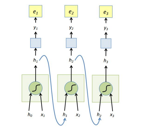
CLICK ME Recurrent Neural Networks (RNN) are designed to analyze sequence data, such as text or time series data. RNNs have shown great success in a wide range of natural language processing tasks, such as speech recognition, machine translation, and text generation. They are also used in many applications related to time series analysis, such as forecasting and trend prediction. A RNN could be represented in a succinct way: The hidden state $h_t$ is decided by $x_t$ and $h_{t-1}$ the hidden state at time $t-1$, $f_w$ injects non-linear weights into $x_t,h_{t-1}$. Classifier usually is a non-linear operation using softmax, assuming the output $y_t$ represents a probability: $$ h_t=tanh(W_x x_t + W_h h_{t-1}) \\ y_t = softmax(W_y h_t) $$ The unfolded graph provides an explicit description of which computations to perform: RNNs are typically trained using backpropagation through time (BPTT), the unfolded network is treated as one big feed-forward network that accepts the whole time series as input. The weight updates are computed for each copy in the unfolded network, then summed or averaged and applied to the RNN weights. Here the loss function we use is cross entroy, and $y_{t_i}$ is the prediction of class $i, i=1,2,...,n$ (assume that we $n$ classes, the dimention of vector $y_t$ is $n \times 1$). $$ E(y,\hat y) = \sum_t E(y_t,\hat y_t) \\ E(y_t,\hat y_t) = - \sum_i \hat y_{t_i} log y_{t_i}\\ \frac{\partial e_3}{\partial W_y}=\frac{\partial e_3}{\partial y_3} \frac{\partial y_3}{\partial W_y}=(\hat y_3 -y_3) \otimes h_3 $$ $\otimes$ is outer product. $$ \begin{aligned} h_t&=tanh(W_x x_t + W_h h_{t-1})\\ \frac{\partial e_3}{\partial W_h} &= \frac{\partial e_3}{\partial y_3} \frac{\partial y_3}{\partial h_3}\frac{\partial h_3}{\partial W_h} \\&=\sum_{k=1}^3 \frac{\partial e_3}{\partial y_3} \frac{\partial y_3}{\partial h_3}\frac{\partial h_3}{\partial h_k}\frac{\partial h_k}{\partial W_h} \end{aligned} $$ The weights $W_h$ are shared and the partial derivative of $e_3$ with respect to $W_h$ is contributed by $h_1,h_2,h_3$. If input sequences are comprised of thousands of timesteps, then the same amount of derivatives required for a single update weight update. This can cause weights to vanish or explode, thus poor model performance. BPTT can be computationally expensive as the number of timesteps increases, as a result, we use truncated BPTT instead: 1. Present a sequence of k1 timesteps of input and output pairs to the network. 2. Unroll the network then calculate and accumulate errors across k2 timesteps. 3. Roll-up the network and update weights. 4. Repeat. Most frequently used RNNs such as LSTM and GRU are not displayed here.
Transformer
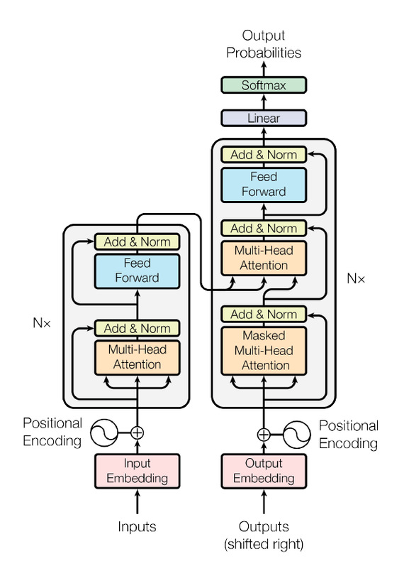
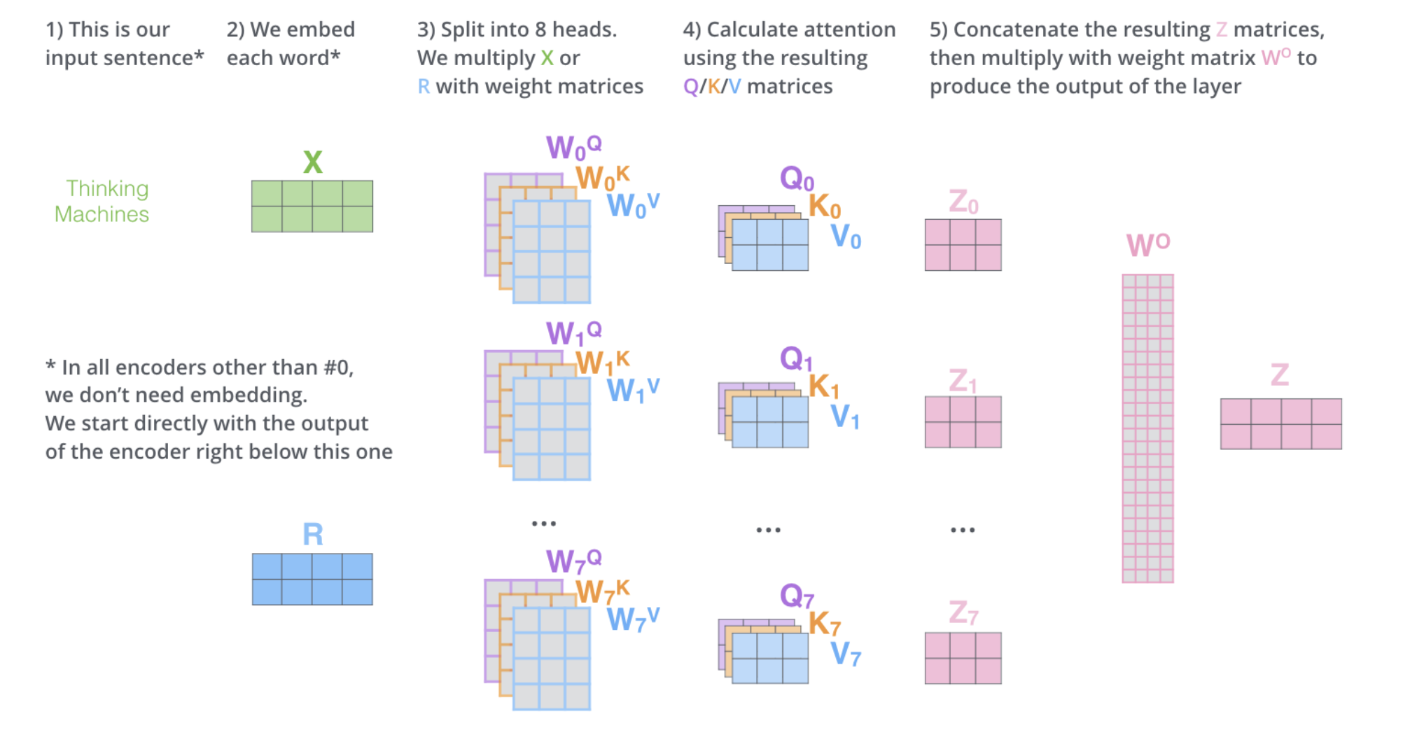
CLICK ME In recent years, transformers has shown it power in natural language process. Applications like Google translate, ChatGPT are based on the transformer architecture, which uses self-attention mechanism to process sequencial data in parallel and catch long-range dependency. RNN has poor parallel capabilities and easily forgets long-distance information, but self-attention overcomes these shortcomings. The attention mechanism allows the model to focus on specific parts of the input sequence and produce a weighted representation of the entire sequence, which can then be used for classification or prediction Let's see what happens to the input text. 1. Each input word is turned into a vector using an embedding algorithm; 2. Create 3 vectors from each input embedding(X), i.e. query(Q), key(K), value(V) by multiplying three matrices learned during the training process. $$ Q=XW^q,K=XW^k,V=XW^v $$ 3. Calculate a attention score for each word/embedding by scaled dot product of query and value matrix, and get the output value matrix of each word, which is then input to the next layer. $$ Score(Q,K)=\frac{QK^T}{\sqrt{d_k}} \\ Output_v(Q,K,V)=softmax(Score(Q,K))V $$ where Score(Q,K) is the attention score and Output_v(Q,K,V) is the output value of the attention layer, $d_k$ is the dimention of key vector. Specificly, the attention score of one word is calculated by sum all dot product between its query and all other key matrices, as displayed below (thanks to the author of this amazing gif): 4. Each sub-layer (self-attention, ffnn) in each encoder has a residual connection around it, and is followed by layer-normalization step. 5. For the original transformer structure which is a encoder-decoder structure, the output of encoders is integrated into the decoder by encoder-decoder attention layer, decoder only structure (GPT) also works perfectly, which reveals the charm of self-attention mechanism. To capture more information in the input text, or gives the attention layer multiple “representation subspaces”, multi-head attention is normally used instead of plain self attention. In essence, we train multiple small weight matrices and concatenate the results into a big matrix. The calculation method of each result is the same as the calculation method of single-head attention. Finally, the generated b is connected to generate the final result. See the Img refered from: http://jalammar.github.io/illustrated-transformer/ . Another blog helps to understand the details of multi-head attention: https://hungsblog.de/en/technology/learnings/visual-explanation-of-multi-head-attention/ Masked Multi-head attention is to force the model to only see the sequence on its left and masks the sequence on its right, which prevent cheating while decoding. In practice, just add negative infinity to each value in the upper triangle part of attention score matrix (excluding diagonal), since softmax will naturally ignore small numbers. The transformer architecture also showed comparable performance to CNN in computer vision tasks after vision transformer (ViT) came out. More details will be added here after further research results appear.
Error state is the difference between True state $x_t$ and Nominal state $x$. The nominal state does not take into account the noise, just derived from motion equations. As a result there will be accumulate errors, which are collected in the error-state $\delta x$ and the ESKF will estimate these errors. In parallel with integration of the nominal state, the ESKF predicts a Gaussian estimate of the error-state, and inject the mean of error state back to nominal-state. When the IMU measurement data arrives, we integrate it and put it into the nominal state variable. Since this approach does not consider noise, the result will naturally drift quickly, so we hope to put the error part as an error variable in ESKF. ESKF will consider the effects of various noises and zero offsets, and give a Gaussian distribution description of the error state. At the same time, ESKF itself, as a Kalman filter, also has a prediction process and a correction process, and the correction process needs to rely on sensor observations other than the IMU. After the correction, ESKF can give the posterior error Gaussian distribution, and then we can put this part of the error into the nominal state variable, and set ESKF to zero, thus completing a loop.
Why ESKF?
CLICK ME In most modern IMU systems, people often use Error state Kalman filter (ESKF) instead of the original state Kalman filter. Since the error-state are small signal, ESKF has several advantages: 1. Regarding of the rotation part, the state variables of ESKF can be expressed by three-dimensional variables, the minimized parameters that are used to express the increment of rotation. While the traditional KF needs to use quaternion (4-dimensional) or higher-dimensional expression (rotation matrix, 9-dimensional), or it has to use a singular expression (Euler angle). 2. ESKF is always near the origin, far away from the singular point, and it will be perfect to perform linearization approximation because it near the operating point. 3. The error-state is always small, meaning that all second-order products are negligible. This makes the computation of Jacobians very easy and fast. 4. The kinematics of the error state is also smaller than the original state variable, because we can put a large number of updated parts into the original state variable.
Equation of State
CLICK ME Good to see all the variables used in a table, all variable names are consistent with the refered Joan's paper: ### Variable List |Magnitude |True |Nominal |Error |Composition|Measured |Noise | | -------- | -------- | -------- | -------- | --------- |-------- |-------- | |Full state| $x_t$ | $x$ | $\delta x$ | $x_t = x \oplus \delta x$ | |Position | $p_t$ | $p$ | $\delta p$ | $p_t = p + \delta p$ | |Velocity | $v_t$ | $v$ | $\delta v$ | $v_t = v + \delta v$ | |Rotation matrix| $R_t$ | $R$ | $\delta R$ | $R_t = R \delta R$ | |Angles vector||| $\delta \theta$ | $\delta R = exp[\delta \theta]$\^ | |Accelerometer bias| $a_{bt}$ | $a_b$ | $\delta a_b$ | $a_{bt} = a_b + \delta a_b$ || $a_\omega$ | |Gyrometer bias|$\omega_{bt}$|$\omega_b$|$\delta \omega_b$|$\omega_{bt} = \omega_b + \delta \omega_b$|| $\omega_\omega$ | |Gravity vector|$g_t$|$g$|$\delta g$|$g_t = g + \delta g$| |Acceleration| $a_t$ |||| $a_m$ | $a_n$ | |Angular rate| $\omega_t$ |||| $\omega_m$ | $\omega_n$ | True state $x_t$ in ESKF: $x_t = [p_t, v_t, R_t, a_{bt}, \omega_{bt}, g_t]^T$, $x_t$ change over time and the subscript $t$ denotes true state. We record the IMU readings as $a_m, \omega_m$, which are perturbed by the white Gaussian noise $a_n, \omega_n$, and $a_\omega$ and $\omega_\omega$ are noise of the bias of IMU. Now we can write the relationship between the derivative of the state variable with respect to the observed measurement (angular velocity is defined in the local reference, the common case in IMU): $$ \dot{p_t} = v_t\\ \dot{v_t} = R_t(a_m-a_{bt}-a_n)+g_t\\ \dot{R_t} = R_t(\omega_m -\omega_{bt}-\omega_n) \hat{} \\ \dot{a_{bt}} = a_\omega\\ \dot{\omega_{bt}} = \omega_\omega \\ \dot{g_t} = 0 $$ Nominal state $x$ kinematics corresponds to the modeled system without noise or perturbations, $$ \dot{p} = v\\ \dot{v} = R(a_m-a_b)+g\\ \dot{R} = R(\omega_m-\omega_b) \hat{}\\ \dot{a_b} = 0\\ \dot{\omega_b} = 0\\ \dot{g_t} = 0 $$ Then we have error state $\delta x$ kinematics: $$ \dot{\delta p} = \delta v \\ \dot{\delta v} = - R(a_m - a_b) \hat{} \delta \theta - R \delta a_b + \delta g - R a_n \\ \dot{\delta \theta} = -(\omega_m - \omega_b) \hat{} \delta \theta - \delta \omega_b - \omega_n \\ \dot{\delta a_b} = a_\omega\\ \dot{\delta \omega_b} = \omega_\omega\\ \dot{\delta g} = 0 $$ The discrete form of error state kinematics: $$ \delta p = \delta p + \delta v \Delta t \\ \delta v = \delta v + (- R(a_m - a_b) \hat{} \delta \theta - R \delta a_b + \delta g) \Delta t + v_i \\ \delta \theta = exp(-(\omega_m-\omega_b)\delta t) \delta \theta - \delta \omega_b \Delta t + \theta_i\\ \delta a_b = \delta a_b + a_i\\ \delta \omega_b = \delta \omega_b + \omega_i\\ \delta g = \delta g $$ where $exp(-(\omega_m-\omega_b)\delta t)$ means the Lie algebra of the incremental rotation, $v_i, \theta_i, a_i, \omega_i$ are the random impulses applied to the velocity, orientation and acceleration and angular rate estimates, modeled by white Gaussian processes. Their mean is zero, and their covariances matrices are obtained by integrating the covariances of $a_n, \omega_n, a_\omega, \omega_\omega$ over the step time $\Delta t$.
Prediction and updating equations
CLICK ME Now we have the motion equation in discrete time domain, $$ \delta x = f(\delta x) + \omega, \omega \sim N(0, Q) $$ $\omega$ is noise, which is composed by $v_i, \theta_i, a_i, \omega_i$ mentioned above, so $Q$ matrix should be: $$ Q = diag(0^3,cov(v_i), cov(\theta_i), cov(a_i), cov(\omega_i),0^3) $$ The prediction equations are written: $$ \delta x_{pred} = F \delta x\\ P_{pred} = FPF^T+Q $$ where $F$ is the Jaccobian of the error state function $f$, the expression is detailed below: $$ \begin{bmatrix} I & I \Delta t &0&0&0&0\\ 0 & I & - R(a_m - a_b) \hat{} \Delta t &-R \Delta t&0&I \Delta t\\ 0&0& exp(-(\omega_m-\omega_b)\Delta t)&0&-I \Delta t&0\\ 0&0&0&I&0&0\\ 0&0&0&0&I&0\\ 0&0&0&0&0&I\\ \end{bmatrix} $$ Suppose an abstract sensor can produce observations of state variables, and its observation equation is written as: $$ z = h(x) + v, v \sim N(0, V) $$ where $h$ is a general nonlinear function of the system state (the true state), and $v$ is measurement noise, a white Gaussian noise with covariance $V$. The updating equations are: $$ K = P_{pred} H^T (H P_{pred} H^T + V)^{-1}\\ \delta x = K (z - h(x_t))\\ P = (I - K H) P_{pred} $$ Where $K$ is Kalman gain, $P_{pred}$ is prediction covariance matrix, $P$ is covariance matrix after updating and $H$ is defined as the Jacobian matrix of measurement equation of error state, according to chain rule $$ H = \frac{\partial h}{\partial \delta x}=\frac{\partial h}{\partial x} \frac{\partial x}{\partial \delta x} $$ First part $\frac{\partial h}{\partial x}$ can be easily obtained by linearizing the measurement equation, the second part $\frac{\partial x}{\partial \delta x}$ is the Jacobian of the true state with respect to the error state, which is the combination of 3x3 identity matrix (for example, $\frac{\partial (p+ \delta p)}{\partial \delta p} = I_3$), expect for the rotation part, in quaternion form it is $\frac{\partial (q \otimes \delta q)}{\partial \delta \theta}$, here in the form of rotation matrix in $SO3$, it is $\frac{\partial log (R Exp(\delta \theta))}{\partial \delta \theta}$, where $Exp(\delta \theta)$ is the Lie algebra of rotation $\delta R$, $H$ can be obtained according to Baker–Campbell–Hausdorff (BCH) formula. Updating the state and reset the error state: $$ x_{k+1} = x_k \oplus \delta x_k\\ \delta x_k = 0 $$ where $\oplus$ is defined addition operation to simplify the following equations: $$ p_{k+1}=p_k+ \delta p_k\\ v_{k+1}=v_k+ \delta v_k\\ R_{k+1}=R_kExp(\delta \theta_k)\\ a_{b,k+1}=a_{b,k}+\delta a_{b,k}\\ \omega_{b,k+1}=\omega_{b,k}+\delta \omega_{b,k}\\ g_{k+1}=g_k+\delta g_k\\ $$
For more derivations and details about quanterion representation in rotation part, please read Joan’s paper: Quaternion kinematics for the error-state Kalman filter, which is also the main reference of this blog.
Kalman Filter (KF) is a recursive state estimator widely used in sensor/data fusion. It’s an optimal Bayesian filter in linear Gaussian system, since it minimizes the estimated error covariance. It is also known as Gaussian Filter. KF is not applicable to discrete or hybrid state spaces. This blog helps understand Kalman Filter with simple examples and presents mathematical derivation from two different perspectives.
Modeling Robot State Estimation
CLICK ME Now we want to estimate the state of a robot <$p, v$>, $p = [p_x, p_y, p_z]^T$ for position and $v = [v_x, v_y, v_z]^T$ for velocity. The state at time $k-1$ is $x_{k-1}=(p_{k-1},v_{k-1})$, we can predict the state at time $k$ if the accelaration $a_k$ is given: $$ p_k = p_{k-1}+v_{k-1} \Delta t + \frac{1}{2}a_k (\Delta t)^2 \\ v_k = v_{k-1}+a_k \Delta t $$ In matrix form: $$ x_k = Ax_{k-1}+Ba_k $$ where $A$ is state transition matrix and $B$ is called control input matrix. $$A = \begin{bmatrix}1 & \Delta t \\ 0 & 1 \end{bmatrix}, B_ = \begin{bmatrix} \frac{1}{2}(\Delta t)^2 \\ \Delta t \end{bmatrix} $$ This is the ideal case. In reality the robot is disturbed by so-called process noise, which models the uncertainty introduced by the state transition. Usually we assume the process noise $\omega_k$ follows a Gaussian distribution (it has to be Gaussian in KF) with zero mean $\omega_k \sim N(0,Q_k)$, $Q_k$ is the covariance matrix. Another observation of the state $z_k$ comes from sensor such as GPS, with measurement noise in Gaussian $v_k \sim N(0, R_k)$. State space model: $$ \begin{aligned} &x_k = Ax_{k-1}+Ba_k+\omega_k \\ &z_k = Hx_k+v_k \end{aligned} $$ where $H_k$ is measurement matrix that map the state space into the observation space.
Mathematical Derivation
Kalman Filter is the optimal filter for Linear Gaussian system, a linear system with almost every variable be Gaussian distributed. KF can be derived in many ways, this section introduces 2 derivations to help better understand KF.
Linear Optimal Estimation How can we guess the real value of $x$ if we observed $x=x_1$ from source 1 and $x=x_2$ from source 2? Theoratically we would never get the real value, but we can approaching the real value or minimize the error between estimated value and real value based on information from different sources under certain assumptions. One option for estimating $x$ is weighted sum of the $x_1$, $x_2$. Kalman Filter corrects the state prediction value according to observed value from sensors to approach the real value, which is similar to weighted sum: $$ \begin{aligned} \tilde{x}_k = \tilde{x}^-_k + K(z_k-H\tilde{x}^-_k) \end{aligned} $$ where $\tilde{x}_k$ is the optimal estimate, $\tilde{x}^-_k$ is predicted state (source 1) and $z_k$ is the observation (source 2). $K$ is called Kalman gain. To determine the value of $K$: $$ \begin{aligned} \tilde{x}_k = &\tilde{x}^-_k + K(Hx_k+v_k-H\tilde{x}^-_k) \\ = &\tilde{x}^-_k + KHx_k+Kv_k-KH\tilde{x}^-_k \end{aligned} $$ subtract $x_k$ from both sides: $$ \tilde{x}_k-x_k = \tilde{x}^-_k-x_k + KH(x_k-\tilde{x}^-_k)+Kv_k $$ Simplify the equation: $$ e_k=x_k-\tilde{x}_k\\ e^-_k=x_k-\tilde{x}^-_k\\ e_k=(I-KH)e^-_k-Kv_k $$ To ensure the estimate $\tilde{x}_k$ is optimal, we have to find the $K$ that minimize $||e_k||^2$, which is equivalent to minimize the trace of covariance matrix $tr(E[e_ke^T_k])$. Set: $$ P_k=E[e_ke^T_k]\\ P^-_k=E[e^-_ke^{-T}_k] $$ Substitute $e_k$: $$ \begin{aligned} P_k=&(I-KH)P^-_k(I-KH)^T+KRK^T\\ =&P^-_k -KHP^-_k-P^-_kH^TK^T+K(HP^-_kH^T+R)K^T \end{aligned} $$ To find the minimum of $tr(P_k)$, we can set the first derivative of $P_k$ with respect to $K$ to 0: $$ \frac{\partial P_k}{\partial K}=-2(P^-_kH^T)+2K(HP^-_kH^T+R)=0\\ K=P^-_kH^T(HP^-_kH^T+R)^{-1} $$ Substituting $K^{-1}P^-_kH^T=HP^-_kH^T+R$ back into the expression of $P_k$: $$ P_k=(I-K_kH)P^-_k $$ We also need to obtain $P^-_k$. Note that noise are independent from the robot state: $$ \begin{aligned} e^-_k=&x_k-\tilde{x}^-_k\\ =&Ax_{k-1}+Bu_k+\omega_k-A \tilde{x}_{k-1}-Bu_k\\ =&A(x_{k-1}-\tilde{x}_{k-1})+\omega_k\\ =&Ae_{k-1}+\omega_k \end{aligned}\\ \begin{aligned} P^-_k=&E[e^-_ke^{-T}_k]\\ =&E[(Ae_{k-1}+\omega_k)(Ae_{k-1}+\omega_k)^T]\\ =&E[(Ae_{k-1})(Ae_{k-1})^T]+E[\omega_k(\omega_k)^T]\\ =&AP_{k-1}A^T+Q \end{aligned}\\ $$ Finally, we can run the Kalman Filter: Step 1. Prediction $$ \tilde{x}^-_k = A\tilde{x}_{k-1}+Ba_k\\ P^-_k = AP_{k-1}A^T+Q $$ Step 2. Measurement update $$ K_k=P^-_kH^T(HP^-_kH^T+R)^{-1}\\ \tilde{x}_k = \tilde{x}^-_k + K(z_k-H\tilde{x}^-_k)\\ P_k=(I-K_kH)P^-_k $$ From the way we find the $K$ for optimal estimation (Least square error), Kalman Filter is the optimal Linear Filter for a Linear system if the noise are independent distributed with zero mean values and valid variances. However, if the system is not a Linear Gaussian, there are non-linear filters perform better than KF, which is another appealing topic. In another word, KF is the optimal estimater for Linear Gaussian System, see the proof below.
Maximum A Posteriori Estimation KF is a Maximum A Posteriori estimator in Linear Gaussian space under Bayesian interpretation following the same 2-step scheme. The goal is finding the $x_k$ to maximize the posterior distribution:$\tilde{x_k}={argmax}_{x_k}\ p(x_k|z_k,a_k)$ Step 1. Prediction: predict $\bar{bel}(x_k)=P(x_k|z_{k-1},a_k)$, the belief of $x_k$ after receiving the control input $a_k$ and before the measurement $z_k$ using the state model, given $bel(x_{t-1})=P(x_{k-1}|z_{k-1},a_{k-1})$, the belief of $x_{k-1}$ (A belief reflects the robot’s internal knowledge about the state of the environment): $$ \begin{aligned} \bar{bel}(x_k)=&P(x_k|z_{k-1},a_k)\\ =&P(x_k|z_{k-1},a_k,a_{k-1})\\ =& \frac{P(x_k,z_{k-1}|a_k,a_{k-1})}{P(z_{k-1})}\\ =& \frac{\int p(x_k,x_{k-1},z_{k-1}|a_k,a_{k-1})dx_{k-1}}{P(z_{k-1})}\\ =& \frac{\int p(x_k|x_{k-1},z_{k-1},a_k,a_{k-1})p(x_{k-1}|z_{k-1},a_{k-1})P(z_{k-1})dx_{k-1}}{P(z_{k-1})}\\ =& \int p(x_k|x_{k-1},a_k)bel(x_{k-1})dx_{k-1}\\ \end{aligned} $$ Note that $x_k$ is only depend on $x_{k-1}$ and $a_k$ (Markov assumption) and $z_{k-1}$ is not dependent on $a_{k-1}$ if $x_{k-1}$ is known (see observation model). $$ bel(x_{k-1}) \sim N(x_{k-1};\mu_{k-1},\Sigma_{k-1})\\ p(x_k|x_{k-1},a_k) \sim N(x_k;Ax_{k-1}+Ba_k,Q_k) $$ The result of multiplying two Gaussian PDFs is in the form of a Gaussion PDF: $$ \bar{bel}(x_{k}) \sim N(x_k;\bar{\mu}_k,\bar{\Sigma}_k)\\ \bar{\mu}_k=A\mu_{k-1}+Ba_k\\ \bar{\Sigma}_k = A\Sigma_{k-1}A^T+Q_k $$ Step 2. Correction / Update: update the prediction using the observation at time $t$ to obtain the estimation $P(x_k|z_k,a_k)$ $$ \begin{aligned} bel(x_k) =&P(x_k|z_k,a_k)\\ =&P(x_k|z_k,z_{k-1},a_k)\\ =& \frac{P(x_k,z_k|z_{k-1},a_k)}{P(z_k|z_{k-1},a_k)}\\ =& \frac{P(z_k|x_k,z_{k-1},a_k)P(x_k|z_{k-1},a_k)}{P(z_k|z_{k-1},a_k)}\\ =& \frac{P(z_k|x_k)\bar{bel}(x_k)}{P(z_k|z_{k-1},a_k)}\\ =& \eta P(z_k|x_k)\bar{bel}(x_k) \end{aligned} $$ Assuming that $z_k$ is independent of previous observations $z_{1:k-1}$, conditional independent of $a_k$ given $x_k$. Normalization factor $\eta$ can be calculated: $$ \begin{aligned} P(z_k|z_{k-1},a_k)=& \int p(z_k,x_k|z_{k-1},a_k)dx_k\\ =& \int p(z_k|x_k,z_{k-1},a_k)p(x_k|z_{k-1},a_k)dx_k \\ =& \int p(z_k|x_k)p(x_k|z_{k-1},a_k)dx_k\\ =& \int p(z_k|x_k)\bar{bel}(x_k)dx_k \end{aligned} $$ Likewise, Two Gaussian PDFs multiplication: $$ p(z_t|x_t) \sim N(z_k;Hx_k,R_k)\\ \bar{bel}(x_{k}) \sim N(x_k;\bar{\mu}_k,\bar{\Sigma}_k)\\ bel(x_{k}) =\eta \exp\{-J_k\} $$ where $$J_k=\frac{1}{2}(z_k-Hx_k)^TR^{-1}_k(z_k-Hx_k)+\frac{1}{2}(x_k-\bar{\mu}_k)^T\bar{\Sigma}^{-1}_k(x_k-\bar{\mu}_k) $$. $J_k$ is quadratic in $x_k$, which means $bel(x_t)$ is a Gaussian. The mean of $bel(x_k)$ is the minimum of this quadratic function, and $bel(x_k)$ reaches it's maximum. After complicated matrix operations and simplification, we will obtain: $$ bel(x_{k}) \sim N(x_k;\mu_k,\Sigma_k)\\ \mu_k=\bar{\mu}_k+K_k(z_k-H\bar{\mu}_k)\\ \Sigma_k = (I-K_kH)\bar{\Sigma}_k\\ K_k=\bar{\Sigma}_kH^T(R_k+H\bar{\Sigma}_kH^T)^{-1} $$ We can use MAP or just use bayesian inference, both works to find the same parameters, since the full Bayesian posterior is exactly Gaussian in a Linear Gaussian system.
A concise definition from T. Mitchell: “A computer program is said to learn from experience E with respect to some class of tasks T and performance measure P, if its performance at tasks in T, as measured by P, improves with experience E”. Regarding of what learning is,Herbert A. Simon once defined it as “the ability that a system improves the performance of itself by executing some process”. Machine learning is a data driven subject that applies machine learning models to data analyzation and prediction. Generally machine learning can be categorized into: supervised learning, unsupervised learning, reinforcement learning, semi-supervised learning and active learning. To design a machine learning system, basically we need to do the following tasks:
Formalize the learning task
Collect data
Extract features
Choose class of learning models
Train model
Evaluate model
This blog revisits some classical supervised learning Models, including K-nearest neighbours, Decision Tree, Naive Bayes, Perceptron and Support Vector Machine.
K-nearest neighbours
CLICK ME Here's how a basic KNN model works in classification tasks: Given a new instance $x_{new}$, find it's K nearest neighbours and then assign $x_{new}$ to the majority class, aka, majority voting (return mean distances from all K instances in regression tasks). We usually pick Euclidean distance to measuring the distance between instances, generally a distance function $d$ should satisfy the following properties: for any instances x, y, z in the sampling set, 1. $d(x, x) = 0;$ 2. $d(x, y) = d(y, x);$ 3. $d(x, y) + d(y, z) ≥ d(x, z);$ Also we'd like to define distance as non-negetive value to avoid troubles, Minkowski distance is the perfect candidate. Good to know some characteristics of k-nearest neighbour learning: 1. Instance-based learning or lazy learning: The model just memorizes training data. Computation is mostly deferred to the classification phase when there is a test example to be processed. Efficient methods such as kd-tree are usually used to accelarate computation speed. 2. Local learner: assumes prediction should be mainly influenced by nearby instances 3. Uniform feature weighting: all features are uniformly weighted in computing distances
Decision Tree
CLICK ME Usually learning a decision tree contains 3 steps: attribute selection, tree generation and pruning. Classical methods such as ID3 (Quinlan 1986), C4-5 (Quinlan 1993) take a greedy top-down learning strategy. For each ndoe, start from the root with full training set and 1. Choose the best attribute to be evaluated; 2. Split node training set into children and form child node according to value of chosen attribute; 3. Stop splitting a node if it contains examples from a single class, or there are no more attributes to test. The best attribute is chosen based on information gain (IG). The IG of attribute A on training dataset D is defined as the difference between the entropy of dataset $H(D)$ and the conditional entropy $H(D|A)$ of D given A. $$ IG(D,A) = H(D)-H(D|A) $$ In information theory, entropy measures the uncertainty of random variables. Given a discrete random variable $X$ that takes a number n of possible values, we have the probability distribution $P$ and entropy $H$: $$ P(X=x_i) = p_i, i = 1, 2, ..., n \\ H(X) = - \sum_{i=1}^n p_i log_2 p_i $$ If we have 2 discrete random variables $(X, Y)$, the conditional entropy $H(Y|X)$ denotes the uncertainty of $Y$ known $X$, as defined below: $$ H(Y|X) = \sum_{i=1}^n p_i H(Y|X=x_i) $$ In classification tasks, the entropy of a set of labelled examples $H(D)$ measures its label inhomogeneity. $H(D|A)$ represents the sum of entropies of subsets of examples obtained partitioning over A values, weighted by their respective sizes. An attribute with high information gain tends to produce homogeneous groups in terms of labels, thus favouring their classification. The information gain criterion tends to prefer attributes with a large number of possible values. Considering an extreme, the unique ID of each example is an attribute perfectly splitting the data into singletons, but it will be of no use on new examples. A measure of such spread is the entropy of the dataset wrt the attribute value instead of the class value. $$ H_A(D) = - \sum_{v \in Values(A)} \frac{\lvert D_v \rvert}{\lvert D \rvert} log_2 \frac{\lvert D_v \rvert}{\lvert D \rvert} $$ The information gain ratio (IGR) measures downweights the information gain by such attribute value entropy. $$ IGR(D, A) = \frac{IG(D, A)}{H_A(D)} $$ Pruing is necessary, since a complex tree can easily overfit the training set, and sometimes requiring that each leaf has only examples of a certain class can lead to very complex trees. It is possible to accept impure leaves, assigning them the label of the majority of their training examples. **Pre-pruning** decides whether to stop splitting a node even if it contains training examples with different labels, while **post-pruning** learns a full tree and successively prune it removing subtrees Usuallly there is a labeled validate set for **post-pruning** to improve the performance of the model. Here's the procedures: 1. For each node in the tree: evaluate the performance on the validation set when removing the subtree rooted at it; 2. If all node removals worsen performance, STOP; 3. Choose the node whose removal has the best performance improvement; 4. Replace the subtree rooted at it with a leaf; 5. Assign to the leaf the majority label of all examples in the subtree; 6. Return to step 1. Decision tree also applies to continuous-valued attributes by discreting the continuous values. Discretization threshold can be chosen in order to maximize the attribute quality criterion (e.g. infogain). Procedure: 1. Examples are sorted according to their continuous attribute values; 2. For each pair of successive examples having different labels, a candidate threshold is placed as the average of the two attribute values; 3. For each candidate threshold, the infogain achieved splitting examples according to it is computed; 4. The threshold producing the higher infogain is used to discretize the attribute;
Naive Bayes
CLICK ME Naive Bayes is a classifier based on Bayes' theorem and conditional probability independence assumption. Each input instance $x$ is described by a conjunction of attribute values $(a_1,..., a_m)$. The output class label belongs to s finite label set $Y$. The task is predicting the MAP target value given the instance $$ \begin{aligned} y^* = argmax_{y_i \in Y}P(y_i|x) & = argmax_{y_i \in Y} \frac{P(a_1,...,a_m|y_i)P(y_i)}{P(a_1,...,a_m)} \\ & = argmax_{y_i \in Y} P(a_1,...,a_m|y_i)P(y_i) \end{aligned} $$ Naive Bayes classifier learns the joint probability distribution of instance and labels, and then predicts the MAP target value for the new instance. However, class conditional probabilities $P(a_1,...,a_m|y_i)$ are hard to learn, as the number of terms is equal to the number of possible instances times the number of target values. Naive Bayes assumption simplifies this problem by assuming that attribute values are independent of each other given the target value: $$ P(a_1,...,a_m|y_i) = \prod_{j=1}^m P(a_j|y_i) \\ y^* = argmax_{y_i \in Y}\prod_{j=1}^m P(a_j|y_i)P(y_i) $$ Thus parameters to be learned reduce to the number of possible attribute values times the number of possible target values. The priors $P(y_i)$ can be learned as the fraction of training set instances having each target value, aka maximum-likelihood estimatimation (MLE), while $P(a_j=v_k|y_i=c)$ can also be learned as the fraction of times the attribute value $v_k$ was observed in training examples of class $c$. Suppose there are N instances in the training set, we have: $$ \begin{aligned} P(a_j=v_k|y_i=c) &= \frac{\sum_{i=1}^N I(a_j=v_k,y_i=c)}{\sum_{i=1}^N I(y_i=c)}\\ &=\frac{N_{kc}}{N_c} \end{aligned} $$ Considering that the probability from MLE could be 0, which would affect the final caculation of Posterior probability and lead to bad results, we use Bayes estimation to add priors of attributes. Assume a Dirichlet prior distribution (with parameters $\alpha_{1c},...,\alpha_{kc}$) for attribute parameters, the posterior distribution for attribute parameters is again multinomial, we have: $$ P(a_j=v_k|y_i=c) = \frac{N_{kc}+\alpha_{kc}}{N_c+\alpha_{c}} $$
Perceptron
CLICK ME Perceptron is a Linear classifier for solving binary classification problems. For training dataset $D$, perceptron learns a hyperplane $\omega x + b=0$ that separates instances: $$ D = \{(x_1,y_1),(x_2,y_2),...,(x_N,y_N)\} \ where\ x_i \in R^n, y_i \in \{-1, +1\}\\ f(x)=sign(\omega x + b) $$ Assume that the dataset is linear separable, i.e. for all instances $x_i$ with positive label $y_i=+1$, $\omega x + b \gt 0$; for all instances $x_i$ with negetive label $y_i=-1$, $\omega x + b \lt 0$. To find the ideal hyperplane, instead of directly minimizing the total number of misclassified instances, perceptron minimize the sum of distances from misclassified instances $x_i \in M$ to the hyperplane. In this case the loss function is continuously differentiable wrt $(\omega,b)$ and can be optimized by Stochastic Gradient Descent (SGD). $$ L(\omega,b)=-\sum_{x_i \in M}y_i(\omega x_i+b) $$ The training procedure: 1. Initialize $\omega_0$, $b_0$; 2. Pick a instance with label $(x_i,y_i)$; 3. If $y_i(\omega x_i+b) \leq 0$, $$ \omega = \omega+\eta x_iy_i \\ b = b+\eta y_i $$ 4. Loop over step 2 ~ 3 until there is no misclassified instance. Note that the ideal hyperplane is not unique, Perceptron could generate different solutions with different initialized $\omega_0$, $b_0$ or non-identical misclassified instances picked during learning.
Support Vector Machine
Linear SVM Support Vector Machine (SVM) is a linear classifier selecting hyperplane maximizing separation margin between classes (large margin classifiers), with solution only depends on a small subset of training examples (support vectors). Considering classifying a linearly separable dataset $Set_{train}$ into 2 classes: $$ Set_{train}: \{(x_1,y_1),(x_2,y_2),...,(x_N,y_N)\} \ where\ x_i \in R^n, y_i \in \{-1, +1\} $$ Usually we will find infinite number of hyperplanes defined by $(\omega, b)$ to seperate the data correctly (e.g. using perceptron), while we can find the optimal hyperplane $(\omega^*, b^*)$ by maximizing the geometric margin $\gamma$: $$ \gamma = \min \gamma_i,\\ \gamma_i = y_i(\frac{\omega}{\lVert \omega \rVert} x_i+ \frac{b}{\lVert \omega \rVert}), i=1,...,N $$ Note that for a certain hyperplane $\omega x_i + b = 0$, the distance between instance $x_i$ and the hyperplane is $\frac{1}{\lVert \omega \rVert} \lvert \omega x_i+ b \rvert$. Large distance denotes high confidence, and label class $y_i$ denotes the correctness of classfication for $x_i$. Finding $(\omega^*, b^*)$ for a hard margin SVM is a constrained optimization problem: $$ \begin{aligned} &\max_{\omega,b} \ \gamma\\ &s.t. \ y_i(\frac{\omega}{\lVert \omega \rVert} x_i+ \frac{b}{\lVert \omega \rVert}) \geq\gamma, i=1,...,N \end{aligned} $$ Substitute geometric margin with $\gamma=\frac{\check{\gamma}}{\lVert \omega \rVert}$, where $\gamma_i$ is the functional margin or confidence margin $\check{\gamma_i}=y_i(\omega x_i+ b)$: $$ \begin{aligned} &\max_{\omega,b} \ \frac{\check{\gamma}}{\lVert \omega \rVert}\\ &s.t. \ y_i(\omega x_i+ b) \geq\check{\gamma}, i=1,...,N \end{aligned} $$ Considering that there is an infinite number of equivalent formulation for the same hyperplane: $$ \begin{aligned} \omega x_i+ b&=0\\ \alpha(\omega x_i+ b)&=0, \ \forall \alpha \neq0 \end{aligned} $$ The canonical hyperplane is the hyperplane having functional/confidence margin equal to 1. We can substitute $\check{\gamma} = 1$ since the problem is equivalent for any $\check{\gamma}$, and convert $\max \frac{1}{\lVert \omega \rVert}$ to its equivalent problem $\min \frac{1}{2} \lVert \omega \rVert ^2$. Now we are dealing with a convex quadratic programming problem (objective is quadratic, points satisfying constraints form a convex set): $$ \begin{aligned} &\min_{\omega,b} \ \frac{1}{2} \lVert \omega \rVert ^2\\ &s.t. \ y_i(\omega x_i+ b)-1 \geq0, i=1,...,N \end{aligned} $$ After solving the convex optimization problem, we will get the hyperplane for separating instances. The hyperplane exists and is unique for a linear separable dataset. $$ \omega^*x+b^*=0\\ f(x)=sign(\omega^*x+b^*) $$ $f(x)$ is the decision function for classification. The above method is maximum margin method, the learning algorithm of Linear SVM. Now let's solve this constrained optimization problem. First build lagrange function: $$ L(\omega,b,\alpha)=\frac{1}{2}\lVert \omega \rVert^2 - \sum_{i=1}^N \alpha_i y_i(\omega x_i+b)+\sum_{i=1}^N \alpha_i \\ \alpha_i \geq 0, i=1,2,...,N $$ where $\alpha_i$ is lagrange multiplier. Considering that we can set $\alpha_i \to +\infty$ for any $\omega,b$ that not satisfy the constraint $ y_i(\omega x_i+ b)-1 \geq0$: $$ \max_{\alpha}L(\omega,b,\alpha)=\begin{cases} \frac{1}{2}\lVert \omega \rVert^2, \text{constraint satisfied}\\ +\infty \end{cases} $$ so the original problem is equivalent to the following problem: $$ \min_{\omega,b} \max_{\alpha}L(\omega,b,\alpha) $$ The Lagrangian is minimized wrt $\omega, b$ and maximized wrt $\alpha_i$ (solution is a saddle point). Usually we tackle this min-max problem by solving its dual problem: $$ \max_{\alpha} \min_{\omega,b}L(\omega,b,\alpha) $$ First, minimize $L(\omega,b,\alpha)$ wrt $\omega,b$ by setting partial derivatives to zero: $$ \frac{\partial}{\partial \omega}L(\omega,b,\alpha)=0 \Rightarrow \omega=\sum_{i=1}^m \alpha_i y_i x_i\\ \frac{\partial}{\partial b}L(\omega,b,\alpha)=0 \Rightarrow \sum_{i=1}^m \alpha_i y_i =0 $$ Substituting in the Lagrangian: $$ \begin{aligned} \min_{\omega,b}L(\omega,b,\alpha)=& \frac{1}{2}\lVert \omega \rVert^2 - \sum_{i=1}^N \alpha_i y_i(\omega x_i+b)+\sum_{i=1}^N \alpha_i \\ =&\frac{1}{2} \sum_{i=1}^N \sum_{j=1}^N \alpha_i \alpha_j y_i y_j(x_i x_j)-\sum_{i=1}^N \alpha_i y_i ((\sum_{j=1}^N \alpha_j y_j x_j)x_i+b)+\sum_{i=1}^N \alpha_i\\ =&-\frac{1}{2} \sum_{i=1}^N \sum_{j=1}^N \alpha_i \alpha_j y_i y_j(x_i x_j)+\sum_{i=1}^N \alpha_i \end{aligned} $$ Then the dual problem is: $$ \begin{aligned} \max_{\alpha} \ &-\frac{1}{2} \sum_{i=1}^N \sum_{j=1}^N \alpha_i \alpha_j y_i y_j(x_i x_j)+\sum_{i=1}^N \alpha_i \\ s.t. \ &\sum_{i=1}^N \alpha_i y_i=0\\ & \alpha_i \geq 0, i=1,2,...,N \end{aligned} $$ Still a constrainted quadratic optimization problem. The solution $(\omega^*,b^*,\alpha^*)$ to the dual problem is the same as the primal problem when Karush-Khun-Tucker (KKT) conditions are satisfied. In this case, KKT conditions: $$ \frac{\partial}{\partial \omega}L(\omega,b,\alpha)=0 \\ \alpha_i^* \geq 0, i=1,2,...,N\\ y_i(\omega^* x_i+b^*)-1 \geq 0, i=1,2,...,N\\ \alpha_i^*(y_i(\omega^* x_i+b^*)-1)=0, i=1,2,...,N\\ $$ From the KKT conditions we know that only points stay on the minimal confidence hyperplane, which are called support vectors, contribute to the final decision function $f(x)$: $$ y_i(\omega^* x_i+b^*)=1 $$ while others points has no contribution since their multiplier have to be zero according to KKT conditions (they could be removed from the training set). SVM are sparse, which means they typically have few support vectors. We notice that dual formulation is easier to solve (simpler constraints) compared with primal formulation. The dual formulation has $N$ variables (number of training examples), while primal formulation has $d + 1$ variables (number of features +1). Depend on the problem, one can choose the primal formulation if it has much less variables. The bias $b$ can be computed from KKT conditions. Given an arbitrary support vector $x_i$ the KKT conditions imply: $$ y_i(\omega^* x_i+b^*)=1\\ b^*=\frac{1-y_i \omega^*x_i}{y_i} $$ For robustness, the bias is usually averaged over all support vectors. We also have the dual SVM decision function by substituting $\omega=\sum_{i=1}^N \alpha_i y_i x_i$: $$ f(x)= sign(\omega x + b)=sign (\sum_{i=1}^N \alpha_i y_i (x_i x)+b) $$ The decision function is a linear combination of dot products between training points and the test point, which denotes the similarity. Weights of the combination are $\alpha_i y_i$: large $\alpha_i$ implies large contribution towards class $y_i$ (times the similarity). The above mentioned SVM is called hard margin SVM, used for dataset that is strictly linear seperable. For linear seperable dataset with outliers, we can still use SVM by adding slack variables to constraints, which is called soft margin SVM.
Non-linear SVM Non-linearly separable problems need a higher expressive power (i.e. more complex feature combinations). Non-linear SVM maps input examples in a higher dimensional feature space where a non-linear problem is transformed into a linear problem, and perform linear classification in this higher dimensional space. $$ \Phi: \mathcal{X} \to \mathcal{H} $$ where $\Phi$ is a function mapping each example in the input space $\mathcal{X}$ to a higher dimensional space $\mathcal{H}$. The feature mapping should increase the expressive power of the representation (e.g. introducing features which are combinations of input features). Examples should be (approximately) linearly separable in the mapped space. SVM algorithm is applied just replacing $x$ with $\Phi(x)$: $$ \begin{aligned} f(x)=& \ \omega \Phi(x)+b \\ =& \sum_{i=1}^N \alpha_i y_i \Phi(x_i) \Phi(x)+b\\ =& \sum_{i=1}^N \alpha_i y_i K(x_i,x)+b \end{aligned} $$ where $K(x_i,x)$ is kernel function, defined as the dot product of $\Phi(x_i)$ and $\Phi(x)$: $$ K(x_i,x)=\Phi(x_i) \Phi(x) $$ Here are several common used kernel functions. 1. polynomial kernel function: $$ K(x,z)=(xz+1)^p $$ 2. Gaussian kernel function: $$ K(x,z)=exp(- \frac{\lVert x-z \rVert ^2}{2 \sigma^2}) $$ SVM also works in regression tasks, this blog will not jump into it.
Logistic Regression
CLICK ME Logistic regression model classify instances based on conditional probability. Here is logistic distribution: $$ F(x)=P(X \leq x)=\frac{1}{1+e^{-(x-\mu) \ / \gamma}}\\ f(x)=\frac{e^{-(x-\mu) \ / \gamma}}{\gamma (1+e^{-(x-\mu) \ / \gamma})^2} $$ Binomial logistic regression model: $$ P(Y=1|x)=\frac{exp(\omega x+b)}{1+exp(\omega x+b)}\\ P(Y=0|x)=1-P(Y=1|x) =\frac{1}{1+exp(\omega x+b)} $$ where $x \in R^n$ is input, $Y \in \{0,1 \}$ is output, $\omega \in R^n$ is weight, $b \in R$ is bias. For convenience, we can simplify the equations as: $$ P(Y=1|x)=\frac{exp(\omega x)}{1+exp(\omega x)}\\ P(Y=0|x)=\frac{1}{1+exp(\omega x)} $$ by setting $\omega = (\omega^{(1)},\omega^{(2)},...,\omega^{(n)},b)^T$, $x=(x^{(1)},x^{(2)},...,x^{(n)},1)^T$. We can tell when the linear combination approaches positive infinity $\omega b \to +\infin$, the conditional probability approaches 1, and vice versa. Learn model parameter $\omega, b$ by maximum likelihood estimation (MLE). Set $$ P(Y=1|x)=\sigma(x), P(Y=0|x)=1-\sigma(x) $$ $$ P(y_i|x_i;\omega)= \begin{cases} \sigma(x_i),y_i=1\\ 1-\sigma(x_i),y_i=0 \end{cases}\\ $$ Rewrite it as: $$ P(y_i|x_i;\omega)=\sigma(x_i)^{y_i}(1-\sigma(x_i))^{1-y_i} $$ Likelihood function: $$ \prod_{i=1}^N \sigma(x_i)^{y_i}(1-\sigma(x_i))^{1-y_i} $$ Log-likelihood function: $$ \begin{aligned} L(\omega)=& \sum_{i=1}^N[y_i log \sigma (x_i)+(1-y_i)log(1-\sigma(x_i))]\\ =& \sum_{i=1}^N[y_i log \frac{\sigma(x_i)}{1-\sigma(x_i)}+log(1-\sigma(x_i))]\\ =&\sum_{i=1}^N[y_i(\omega x_i)-log(1+exp(\omega x_i))] \end{aligned} $$ Maximize $L(\omega)$ to find $\omega$ using gradient descent or Newton method. Multi-nominal logistic regression model for multi-class classification task, suppose we have $K$ classes $Y \in \{ 1,2,...,K \}$: $$ P(Y=k|x)=\frac{exp(\omega_k x)}{1+\sum_{k=1}^{K-1}exp(\omega_k x)}, k = 1,2,...,K-1\\ P(Y=K|x)=\frac{1}{1+\sum_{k=1}^{K-1}exp(\omega_k x)} $$ where $x \in R^{n+1}$, $\omega_k \in R^{n+1}$. Parameter estimation follows the same scheme in binomial logistic regression model.
Git is a distributed version control tool that runs on Linux, Unix, Mac and Windows. With the help of Git, you don’t have to manually record and save copies every time when the files are changed, or worry about file exchange and protection when working on big projects with others. This post introduces common usage of Git.
Large Language Models (LLM) have surprised us in many ways, such as talking like human, processing paper work, codeing copilot, analyzing data…, simply by predicting the next token using probability model. As the LLMs get smarter and lighter, we can leverage LLMs that are close to or even surpasse the capabilities of ChatGPT on our device, which is going to make our life much easier. This blog shows how to build a chatbot that runs 100% locally and shares my thoughts on how the LLMs can help in our daily life.
This blog post go through the basics of point cloud data and related projects I have done, including point cloud registration, point cloud segmentation.
This is a blog post that records the steps to set environment before I successfully trained and run a deep learning model in a docker container. Docker offers an isolated environment for software and dependencies and ensure the application runs quickly and reliably from one computing environment to another, by using container technology. See the difference between docker container and virtual machine in https://www.docker.com/resources/what-container/. Have docker installed on the host computer, build docker environment following steps below.
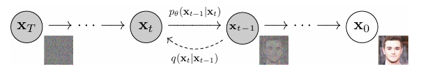
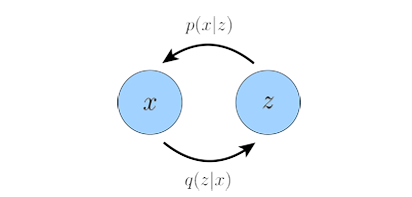
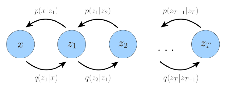
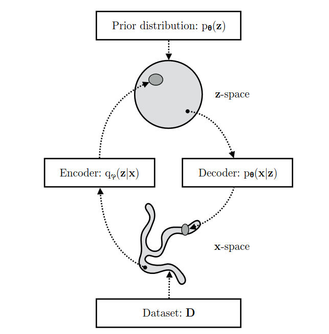
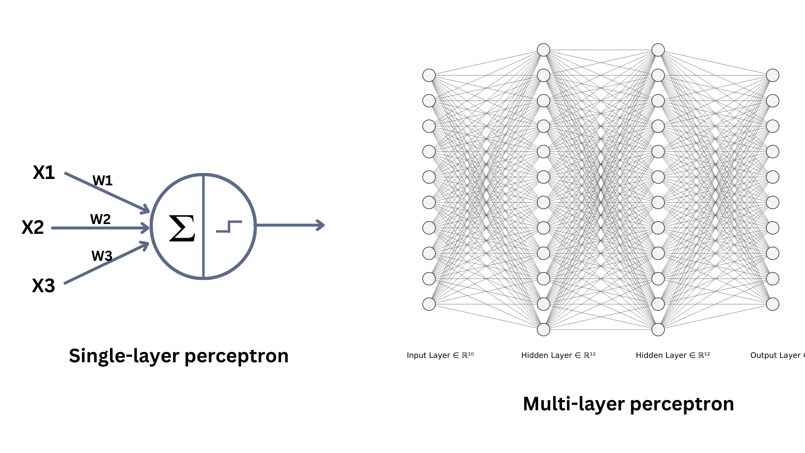
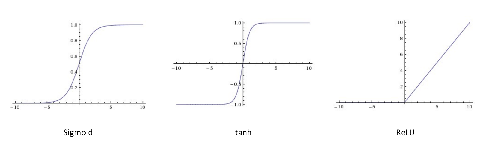
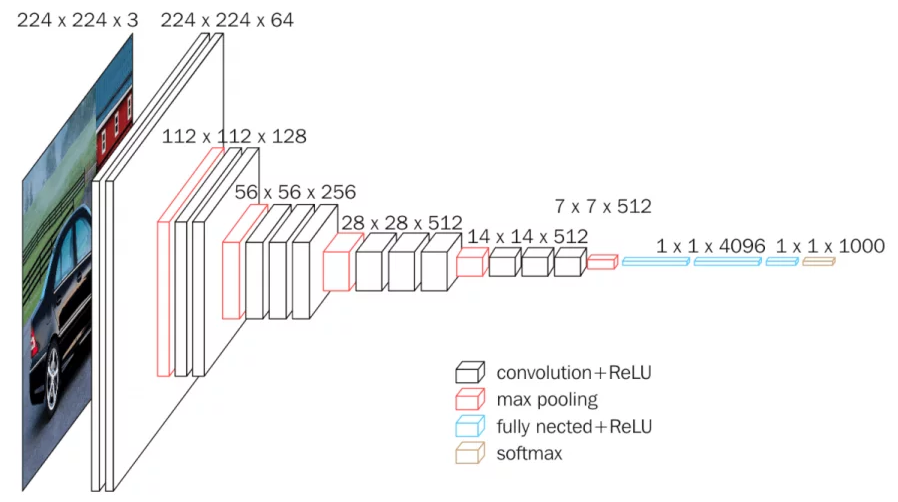
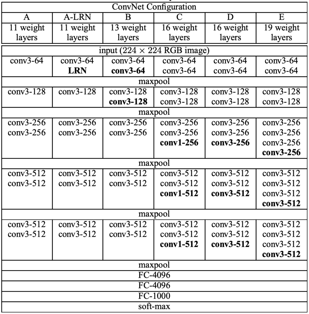
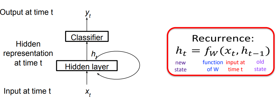
.png)